

Hiveplotlib v0.27.0 Speedups#
This post documents performance improvements in Hiveplotlib v0.27 when generating hive plots for large networks.
These improvements were driven primarily by:
Speeding up edge construction via Numba JIT compilation and parallelization.
Improved bookkeeping when plotting with the
datashaderback end.Lowered DPI when plotting with the
datashaderback end.
Key Takeaways#
1. Hiveplotlib is faster for large networks#
Runtimes for both hive plot building and plotting have dropped dramatically for larger hive plots.
2. No user API changes required#
If Numba is installed, you will automatically get the speedups when you install the newer version of Hiveplotlib. If desired, you can still force edge construction to run single-threaded / without Numba acceleration.
3. Hiveplotlib is not requiring Numba with these changes#
If Numba is not available, Hiveplotlib will fall back to using non-accelerated edge construction.
What Changed#
These changes targeted the two primary runtime constraints: edge construction and rendering figures. Note, the rendering accelerations only apply to plotting with the datashader back end.
Edge Construction#
Added JIT-compilation via Numba (when available), using
nopythonandfastmathmodes, which now run by default.Added parallelization with Numba
prangefor embarrassingly parallel edge assembly (when available), using all available threads by default. When the workload is small (fewer total sampled points), a serial Numba implementation is used instead to avoid the overhead of thread coordination.Reduced edge floating point precision (
float64tofloat32) to save time and memory.
Rendering Figures#
Reduced unnecessary DataFrame construction when aggregating edges for datashading. Previously, each axis pair’s edge curves were wrapped in a separate DataFrame before concatenation; now, raw arrays are concatenated once and a single DataFrame is built at the end.
Only the edge/node metadata column required by the chosen Datashader reduction is carried through the aggregation, rather than all metadata columns.
Lower default DPI using the
datashaderback end leads to less bin values to compute and thus faster rendering.
Methodology for Assessing Runtime#
We ran the following profiling exercise to generate the plots below:
Generate a hive plot with \(n\) nodes and \(e\) edges, tracking the total hive plot build time.
Visualize this hive plot using the
datashaderback end, tracking the total time to render the hive plot visualization.Run this exercise for the chosen \((n, e)\) combination a total of five times.
We then plot the mean runtime (in seconds) for each \((n, e)\) as a heat map, with a separate heat map for build time and plotting time.
Each heat map considers 16 different node counts x 16 different edge counts ranging from 1000 to 1,000,000 nodes / edges, for a total of 256 distinct hive plots (where each hive plot was constructed and plotted five times, so 1280 total runs per heat map).
Build Time Improvements#
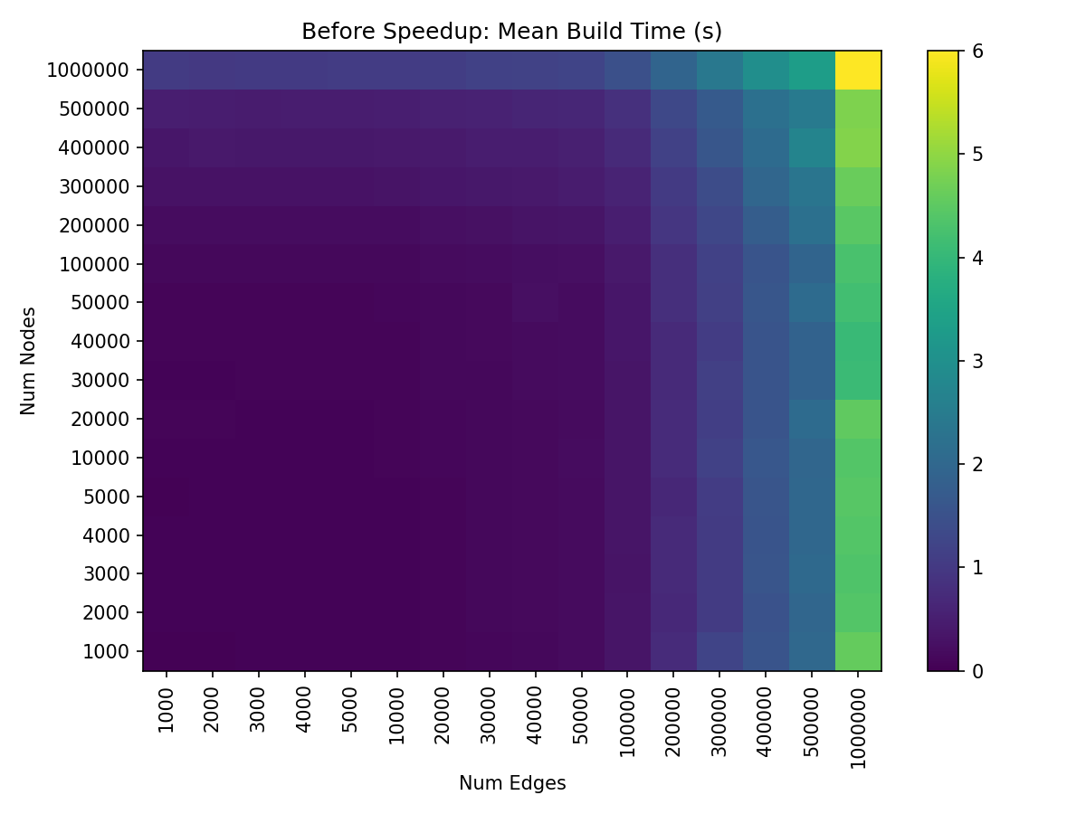
Edge construction was originally a much larger runtime bottleneck than node construction, as demonstrated by the relatively consistent color of each column.
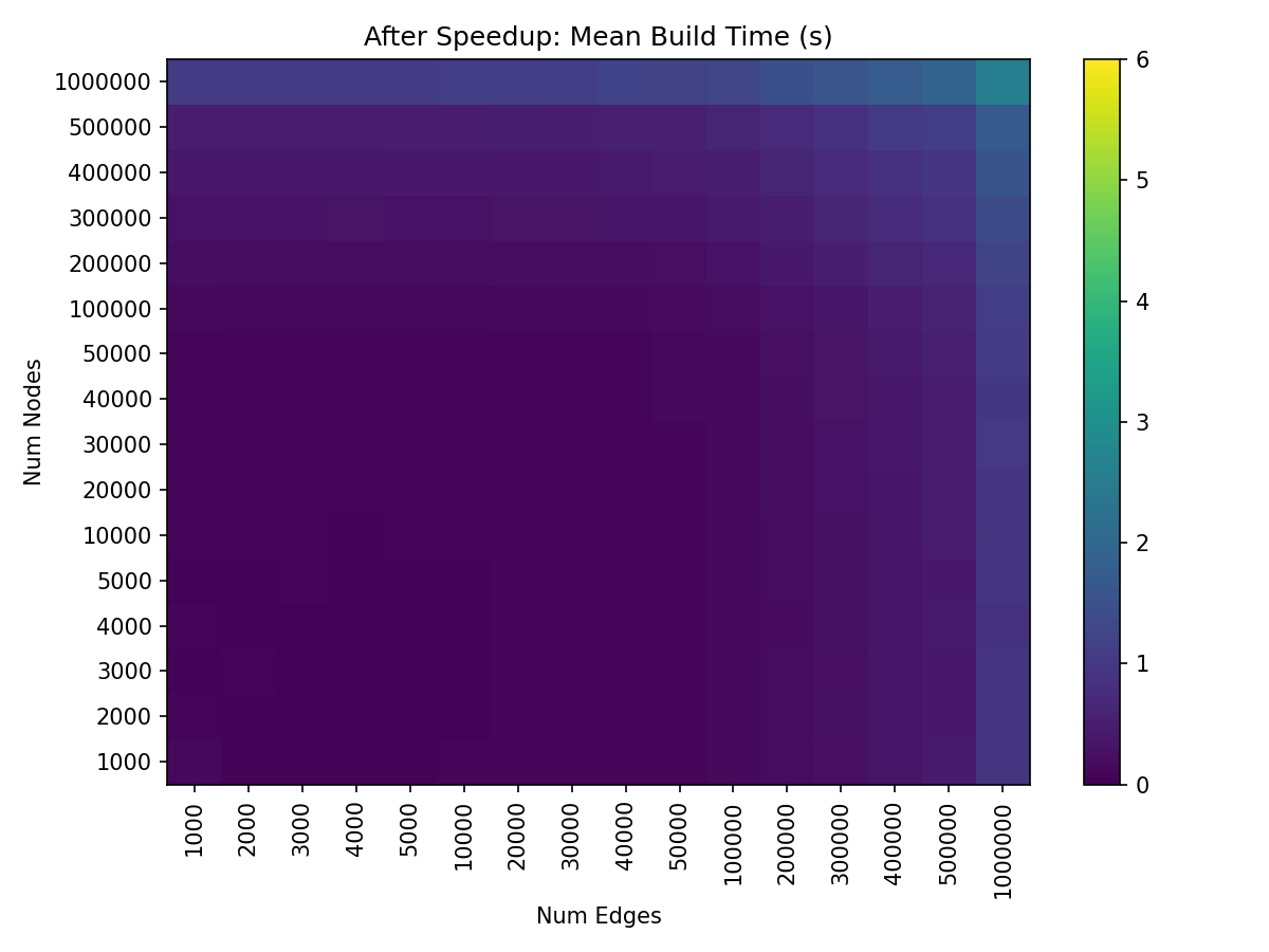
After speeding up edge construction, build time is roughly equally constrained by the number of edges / nodes.
With these improvements to edge construction, overall hive plot build time on our test machine is now running in roughly half the time for larger hive plots without any notable sacrifices when building smaller hive plots.
Visualization Time Improvements#
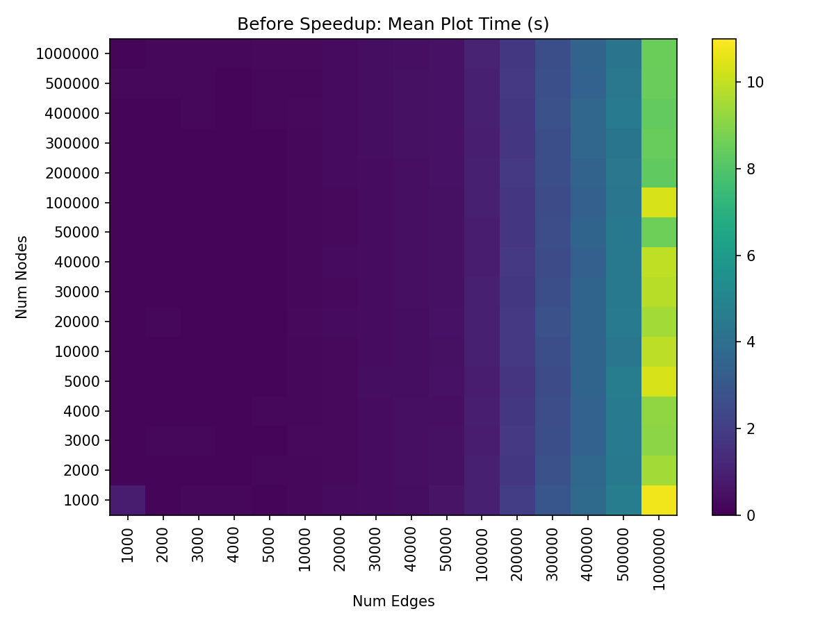
Larger numbers of edges are the bottleneck to plotting, as demonstrated by the relatively consistent color of each column.
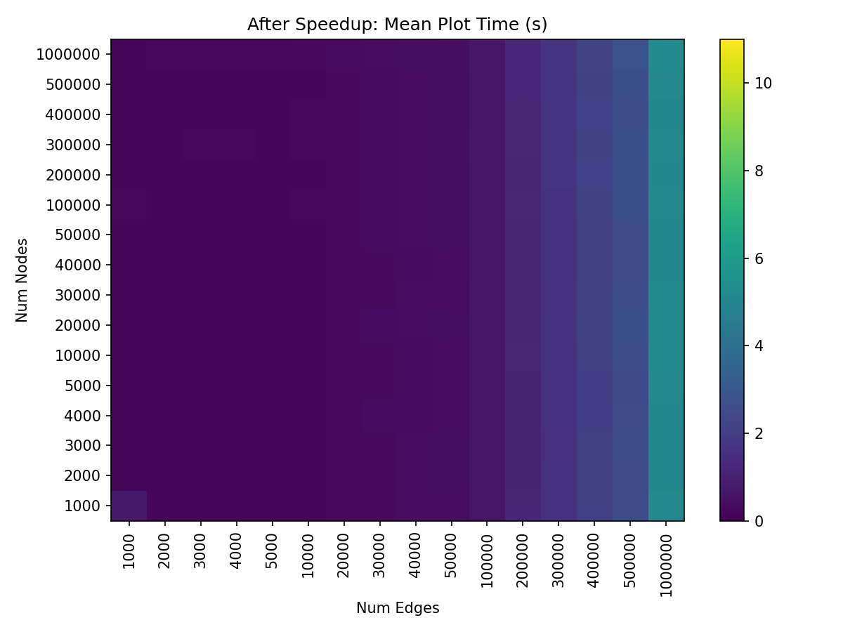
After speeding up edge plotting, plot time is still bottlenecked by edges, but nonetheless dramatically sped up compared to before.
(Note this figure was generated using a fixed dpi=300 when rendering each hive plot. We’ll talk more about speedups via changing the dpi default in the next section.)
With these improvements to edge plotting, overall hive plot visualization time on our test machine also now runs in roughly half the time for larger hive plots without any notable sacrifices when plotting smaller hive plots.
Additional Visualization Time Improvements (Lowered DPI)#
Plotting with the datashader back end can be slowed noticeably by our choice of the dpi parameter, which dictates the size of the rasterization (for more information on how the datashader back end works with respect to dpi, see the Datashader page).
Higher dpi results in a higher resolution visualization, but at the cost of longer rendering time.
In this release, we’ve lowered the default dpi from 300 to 150. With lower dpi, we were also able to lower the default pixel_spread_nodes and pixel_spread_edges values for node and edge visualizations, respectively, which further speeds up the visualization.
The result is a comparable figure generated noticeably faster than was possible with the previous default parameters, albeit at lower-resolution.
These new default values can always be increased if a user needs a particularly high-resolution figure by setting them when plotting a HivePlot instance (hp):
hp.set_viz_backend("datashader")  # make sure you're using the datashader back end
hp.plot(
    dpi=<new dpi>,                          # new default is 150
    pixel_spread_nodes=<new node spread>,   # new default is 7
    pixel_spread_edges=<new edge spread>,   # new default is 1
)
To demonstrate the speedup, let’s make a quick example hive plot with a large number of random nodes and edges:
[1]:
from hiveplotlib.datasets import example_hive_plot
import matplotlib.pyplot as plt

hp = example_hive_plot(
    num_nodes=100000,
    num_edges=100000,
    backend="datashader",
)
When we visualize it using our old default parameters, we get the following run times:
[2]:
%%timeit
fig, ax, _, _ = hp.plot(
    dpi=300,                # new default is 150
    pixel_spread_nodes=15,  # new default is 7
    pixel_spread_edges=2,   # new default is 1
)
plt.close(fig)
508 ms ± 9.32 ms per loop (mean ± std. dev. of 7 runs, 1 loop each)
But when we visualize it with our new default parameters, we see a substantial speedup:
[3]:
%%timeit
fig, ax, _, _ = hp.plot()  # new defaults
plt.close(fig)
305 ms ± 8.78 ms per loop (mean ± std. dev. of 7 runs, 1 loop each)
To demonstrate how similar the visualizations look, below we generate another example hive plot and visualize it using the old and new default parameters:
[4]:
hp = example_hive_plot(
    num_nodes=1000,
    num_edges=1000,
    backend="datashader",
)

# previous default parameters
fig, ax, _, _ = hp.plot(
    dpi=300,                # new default is 150
    pixel_spread_nodes=15,  # new default is 7
    pixel_spread_edges=2,   # new default is 1
)

ax.set_title("Previous Default DPI Parameters")

# new default parameters
fig, ax, _, _ = hp.plot()

ax.set_title("New Default DPI Parameters")

plt.show()
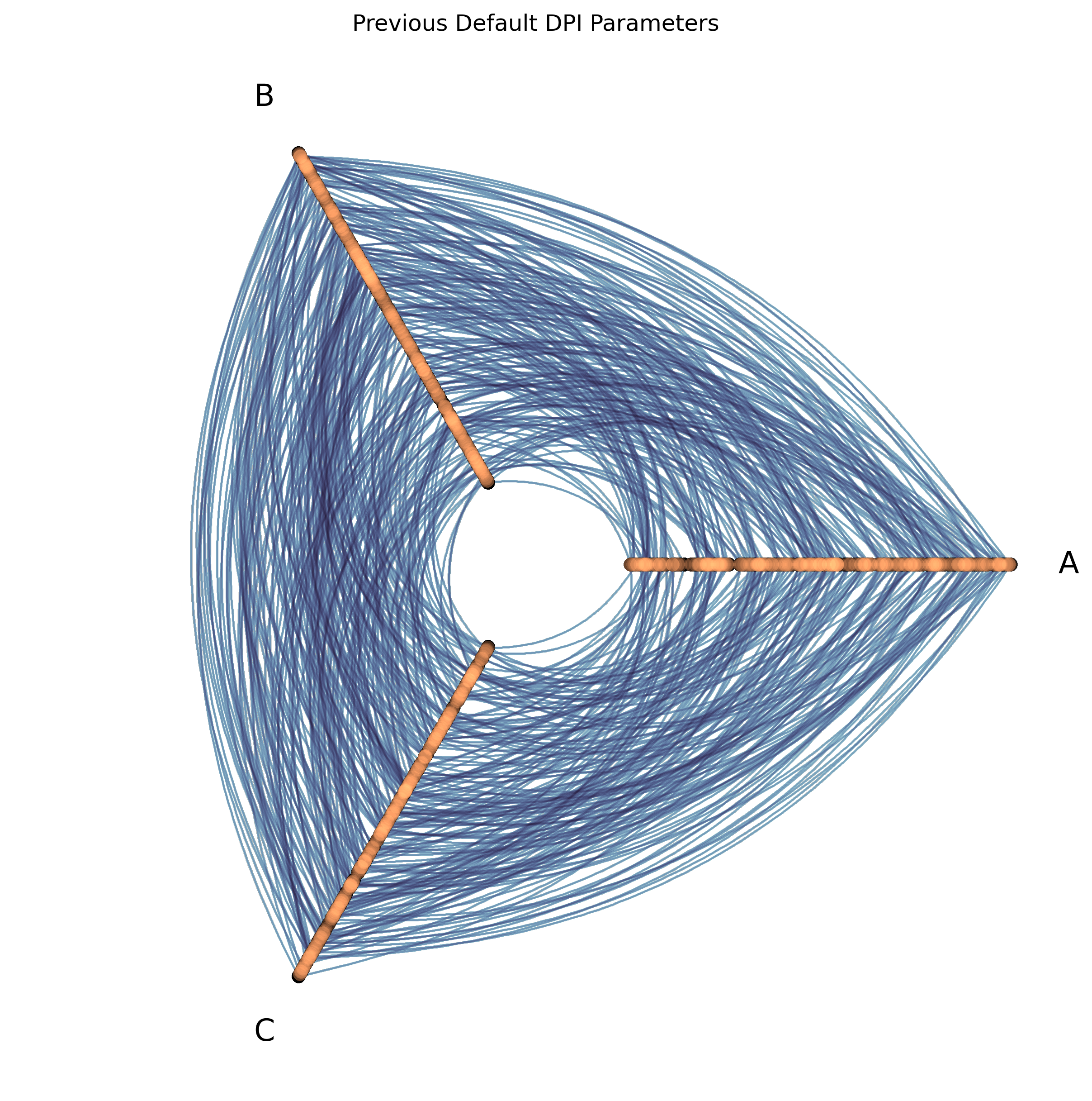
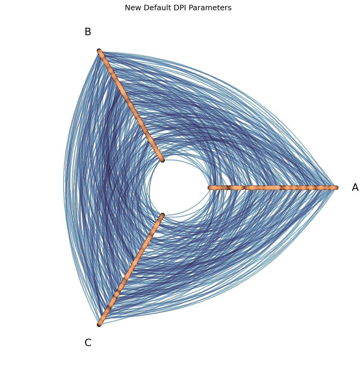
Almost identical!
Datashader Viz Using the Previous DPI Defaults#
To restore the previous default paramaters in this new release of Hiveplotlib, users can manually set the relevant parameters when plotting their HivePlot instance (hp):
hp.set_viz_backend("datashader")  # make sure you're using the datashader back end
hp.plot(
    dpi=300,                # new default is 150
    pixel_spread_nodes=15,  # new default is 7
    pixel_spread_edges=2,   # new default is 1
)
This Is Not a Breaking Change!#
Numba is not required with these changes. If Numba is not available, Hiveplotlib will fall back to non-accelerated edge construction.
New Default Behavior / Parameters#
If numba is not available in your Python environment, then you should not observe any speedup in hive plot build times.
if you are using the hiveplotlib[datashader] back end, then numba is already installed as a dependency, and upgrading your Hiveplotlib installation will run the Numba-accelerated hive plot build process.
Opt Out of Numba Use with use_numba#
If you want to opt out entirely of using Numba acceleration in your hive plot build, you can set use_numba=False when instantiating your HivePlot object. This new parameter defaults to True as of Hiveplotlib 0.27.0.
Constrain the Number of Threads with n_parallel#
If you want to constrain how many threads are used in parallel edge construction, you can set n_parallel=<int> when instantiating your HivePlot object. This new parameter defaults to None (which uses all available CPU cores, capped by the number of curves) as of Hiveplotlib 0.27.0.
Note that n_parallel sets a process-global Numba thread count. If you are building multiple HivePlot instances concurrently from different threads, be aware that the thread count setting is not thread-safe.
Notes#
This was run on a desktop computer with 24 available threads; speedups will vary based on each user’s hardware.
If you run into any unexpected problems from this change, please let us know by opening an issue.