P2CPs Using Other Visualization Libraries

This notebook first demonstrates how to visualize P2CPs with bokeh and plotly through formal hiveplotlib support.

We then show how to create a baseline JSON output from a toy P2CP instance.

Finally, we demonstrate how to visualize this toy P2CP in pure matplotlib. Although hiveplotlib of course supports matplotlib visualizations formally, this last example is meant to demonstrate wrangling the JSON data product to help users who need to translate the JSON output to an unsupported Python visualization library.

import json

import matplotlib.pyplot as plt
import numpy as np
from hiveplotlib import p2cp_n_axes
from hiveplotlib.datasets import four_gaussian_blobs_3d
from hiveplotlib.utils import cartesian2polar, polar2cartesian
from hiveplotlib.viz import p2cp_legend, p2cp_viz
from matplotlib.collections import LineCollection

Matplotlib Baseline

We will use the following example throughout this notebook, which is a simplified version of the example covered in the Introduction to P2CPs notebook.

# fix color dict (for better replication of figures between viz libraries)
color_dict = dict(zip(range(4), ["#0173b2", "#de8f05", "#029e73", "#cc78bc"]))


df = four_gaussian_blobs_3d(num_points=2)

p2cp = p2cp_n_axes(data=df, split_on="Label", vmins=[-1] * 3, vmaxes=[6] * 3)

# set colors according to above-defined color dictionary
#  (so we can replicate more easily in other viz later)
for tag in color_dict:
    p2cp.add_edge_kwargs(tag=tag, color=color_dict[tag])
fig, ax = p2cp_viz(p2cp, node_kwargs={"s": 20, "alpha": 1}, alpha=1, lw=4)
p2cp_legend(p2cp, fig=fig, ax=ax, line_kwargs={"lw": 4})

ax.set_title("Hiveplotlib Starting Point", fontsize=20)
plt.show()

bokeh

hiveplotlib supports visualizations with a bokeh backend, mirroring the same function calls as the matplotlib-based functions. One need only switch the import from hiveplotlib.viz to hiveplotlib.viz.bokeh.

Note: the hiveplotlib.viz.bokeh module requires that hiveplotlib be installed with the bokeh package, which can be done by running:

$ pip install hiveplotlib[bokeh]

from bokeh.io import output_notebook
from bokeh.plotting import show
from hiveplotlib.viz.bokeh import p2cp_legend, p2cp_viz

output_notebook()

Loading BokehJS ...

fig = p2cp_viz(
    p2cp,
    axes_kwargs={"line_alpha": 1, "line_width": 2},
    axes_labels_fontsize="16px",
    line_width=3,
    line_alpha=1,
)
fig.title = "Hiveplotlib (Bokeh Backend)"
fig.title.text_font_size = "30px"
p2cp_legend(p2cp, fig=fig)
show(fig)

plotly

hiveplotlib supports visualizations with a plotly backend, mirroring the same function calls as the matplotlib-based functions. One need only switch the import from hiveplotlib.viz to hiveplotlib.viz.plotly.

Note: the hiveplotlib.viz.plotly module requires that hiveplotlib be installed with the plotly package, which can be done by running:

$ pip install hiveplotlib[plotly]

import plotly.io
from hiveplotlib.viz.plotly import p2cp_legend, p2cp_viz

plotly.io.renderers.default = "plotly_mimetype+notebook"

fig = p2cp_viz(p2cp, opacity=1, line_width=3)
p2cp_legend(p2cp, fig=fig)
fig.update_layout(title={"text": "Hiveplotlib (Plotly Backend)", "font": {"size": 30}})
fig

Exporting P2CPs as JSON

To accommodate any library / language one might choose for the final visualization of their P2CP, we support exporting the relevant data as JSON via the hiveplotlib.P2CP.to_json() method.

To pull out the information of this P2CP instance, we simply need to call the P2CP.to_json() method.

p2cp_json = p2cp.to_json()

What’s in the Output JSON

P2CP.to_json() creates the following JSON structure:

{
  "axes": {
    "<axis_id_0>": {
      "start": [axis_id_0_start_x (float), axis_id_0_start_y (float)],
      "end": [axis_id_0_end_x (float), axis_id_0_end_y (float)],
      "points: {
        "unique_id": [list, of, unique, point, ids],
        "x": [list, of, corresponding, point, x, values],
        "y": [list, of, corresponding, point, y, values]
      }
    },
       .
       .
       .
    "<axis_id_n>": {
      ...
    }
  }
  "edges": {
    "tag": {
      "ids": [point_0_id, ... , point_k_id],
      "edge_kwargs": {<matplotlib edge kwargs>},
      "curves": {
        "from_axis_id": {
          "to_axis_id": [[edge_0_x_0, edge_0_y_0], ... , [edge_0_x_j, edge_0_y_j],
                        [null, null],
                        [edge_1_x_0, edge_1_y_0], ... , [edge_1_x_j, edge_1_y_j],
                        [null, null],
                             .
                             .
                             .
                        [edge_k_x_0, edge_k_y_0], ... , [edge_k_x_j, edge_k_y_j]]
        }
      }
    }
  }
}

The highest-level separation is the top-level keys "axes" and "edges".

Axis and Point Information

"axes" contains the start and end points of each axis in Cartesian space, as well as the IDs and corresponding Cartesian coordinates of each point on a given axis.

For example, the information about axis "A" is under ["axes"]["A"], and the information for the points on axis "A" is under:

["axes"]["A"]["points"].

Edge Information

"edges" contains the discretized curve information for plotting edges.

Organized by nested dictionaries, the edges are split up first by which tag of points they correspond to, that is, the edges of points whose IDs are under:

["edges"][<tag>]["ids"]

are all stored within ["edges"][<tag>]["curves"].

Amongst that subset of curves, all the edges that go from axis "A" to axis "B" are stored under:

["edges"][<tag>]["curves"]["A"]["B"].

Note: all those curves going from one axis to another axis with the same tag are stored together in a single data structure. The breakpoint between each of these curves in JSON is a [null, null] value. (Recasting these null values to np.nan in Python allows for much faster, single-layer plotting in matplotlib, plotly, and holoviews.)

Any corresponding matplotlib kwargs generated along the way for a given tag of data are preserved under:

["edges"][<tag>]["edge_kwargs"].

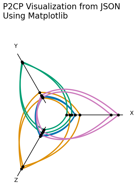
Replicating our Matplotlib Viz from JSON

Once we read the JSON back into Python as a dict, we can manually plot in matplotlib without touching the hiveplotlib.viz module.

# read in JSON output that we exported from `P2CP` instance above
p2cp_dict = json.loads(p2cp_json)

fig, ax = plt.subplots(figsize=(6, 6))

for axis in p2cp_dict["axes"]:
    # plot axis
    axis_start = p2cp_dict["axes"][axis]["start"]
    axis_end = p2cp_dict["axes"][axis]["end"]
    axis_range = np.row_stack([axis_start, axis_end])
    ax.plot(axis_range[:, 0], axis_range[:, 1], color="black")

    # plot points
    points = p2cp_dict["axes"][axis]["points"]
    ax.scatter(points["x"], points["y"], color="black", zorder=2)

    # add axis labels
    #  grab each endpoint, and move out in polar space to space away from axes
    rho, phi = cartesian2polar(x=axis_end[0], y=axis_end[1])
    new_x, new_y = polar2cartesian(rho=rho + 0.5, phi=phi)
    ax.text(s=axis, x=new_x, y=new_y, size=14)

# plot edges
for tag in p2cp_dict["edges"]:
    # only plot if there are curves generated
    if "curves" in p2cp_dict["edges"][tag]:
        for edge_from in p2cp_dict["edges"][tag]["curves"]:
            for edge_to in p2cp_dict["edges"][tag]["curves"][edge_from]:
                curves_to_plot = np.array(
                    p2cp_dict["edges"][tag]["curves"][edge_from][edge_to]
                ).astype(float)
                # if there's no actual edges there, don't plot
                if curves_to_plot.size > 0:
                    split_arrays = np.split(
                        curves_to_plot, np.where(np.isnan(curves_to_plot[:, 0]))[0]
                    )
                    for_stacking = [
                        i[np.where(~np.isnan(i[:, 0]))[0], :]
                        for i in split_arrays
                        if i.shape[0] > 1
                    ]
                    stacked = np.stack(for_stacking, axis=0)
                    collection = LineCollection(
                        stacked, lw=3, zorder=1, color=color_dict[int(tag)]
                    )
                    ax.add_collection(collection)


ax.set_title(
    "P2CP Visualization from JSON\nUsing Matplotlib", x=0, y=1.2, size=20, ha="left"
)
ax.axis("off")
ax.axis("equal")
plt.show()

Holoviews P2CPs from JSON

Holoviews can follow the same data wrangling as the pure matplotlib visualization. Below, we demonstrate using both the bokeh and matplotlib backends.

Holoviews (Bokeh Backend)

import holoviews as hv

hv.extension("bokeh")

# read in JSON output that we exported from `P2CP` instance above
p2cp_dict = json.loads(p2cp_json)

curve_plots = []
# plot edges first for ordering
for tag in p2cp_dict["edges"]:
    # only plot if there are curves generated
    if "curves" in p2cp_dict["edges"][tag]:
        for edge_from in p2cp_dict["edges"][tag]["curves"]:
            for edge_to in p2cp_dict["edges"][tag]["curves"][edge_from]:
                curves_to_plot = np.array(
                    p2cp_dict["edges"][tag]["curves"][edge_from][edge_to]
                ).astype(float)

                # break apart each curve array
                split_arrays = np.split(
                    curves_to_plot, np.where(np.isnan(curves_to_plot[:, 0]))[0]
                )
                temp_curves = [
                    hv.Curve(c).opts(color=color_dict[int(tag)], line_width=3)
                    for c in split_arrays
                ]
                curve_plots += temp_curves

axis_plots = []
point_plots = []
annotation_plots = []
for axis in p2cp_dict["axes"]:
    # plot axis
    axis_start = p2cp_dict["axes"][axis]["start"]
    axis_end = p2cp_dict["axes"][axis]["end"]
    axis_range = np.row_stack([axis_start, axis_end])
    axis_plots.append(hv.Curve(axis_range).opts(color="black"))

    # plot points
    points = p2cp_dict["axes"][axis]["points"]
    point_plots.append(
        hv.Points(np.c_[points["x"], points["y"]]).opts(color="black", size=5)
    )

    # add axis labels
    #  grab each endpoint, and move out in polar space to space away from axes
    rho, phi = cartesian2polar(x=axis_end[0], y=axis_end[1])
    new_x, new_y = polar2cartesian(rho=rho + 0.5, phi=phi)
    annotation_plots.append(hv.Text(new_x, new_y, axis))

fig = hv.Overlay(curve_plots + axis_plots + point_plots + annotation_plots).opts(
    height=500,
    width=500,
    title="P2CP Visualization from JSON\nUsing Holoviews (Bokeh Backend)",
    padding=0.1,
    xaxis=None,
    yaxis=None,
    aspect="equal",
)
fig

Holoviews (Matplotlib Backend)

import holoviews as hv

hv.extension("matplotlib")

# read in JSON output that we exported from `P2CP` instance above
p2cp_dict = json.loads(p2cp_json)

curve_plots = []
# plot edges first for ordering
for tag in p2cp_dict["edges"]:
    # only plot if there are curves generated
    if "curves" in p2cp_dict["edges"][tag]:
        for edge_from in p2cp_dict["edges"][tag]["curves"]:
            for edge_to in p2cp_dict["edges"][tag]["curves"][edge_from]:
                curves_to_plot = np.array(
                    p2cp_dict["edges"][tag]["curves"][edge_from][edge_to]
                ).astype(float)

                # break apart each curve array
                split_arrays = np.split(
                    curves_to_plot, np.where(np.isnan(curves_to_plot[:, 0]))[0]
                )
                temp_curves = [
                    hv.Curve(c).opts(color=color_dict[int(tag)]) for c in split_arrays
                ]
                curve_plots += temp_curves

axis_plots = []
point_plots = []
annotation_plots = []
for axis in p2cp_dict["axes"]:
    # plot axis
    axis_start = p2cp_dict["axes"][axis]["start"]
    axis_end = p2cp_dict["axes"][axis]["end"]
    axis_range = np.row_stack([axis_start, axis_end])
    axis_plots.append(hv.Curve(axis_range).opts(color="black"))

    # plot points
    points = p2cp_dict["axes"][axis]["points"]
    point_plots.append(
        hv.Points(np.c_[points["x"], points["y"]]).opts(color="black", s=30)
    )

    # add axis labels
    #  grab each endpoint, and move out in polar space to space away from axes
    rho, phi = cartesian2polar(x=axis_end[0], y=axis_end[1])
    new_x, new_y = polar2cartesian(rho=rho + 0.5, phi=phi)
    annotation_plots.append(hv.Text(new_x, new_y, axis))

hv.Overlay(curve_plots + axis_plots + point_plots + annotation_plots).opts(
    fig_size=200,
    title="P2CP Visualization from JSON\nUsing Holoviews (Matplotlib Backend)",
    xaxis=None,
    yaxis=None,
    aspect=0.9,  # default aspect was squeezing figure for reasons unknown
    padding=0.1,
    fontsize={"title": "xx-large"},
)