Hive Plot Matrices

A single hive plot best-handles networks with up to 3 groups, with the 3-axis layout showing every pairwise relationship without overlap. But what should we do when our network partitions into more than 3 groups? What if we want to compare how different partition variables and sorting variables reshape the plot? Or what if we want to independently explore distinct subsets of edges?

How can we systematically explore a network that exceeds the optimal capacity of a single hive plot?

The answer Hiveplotlib offers is the Hive Plot Matrix (HPM): a matrix of small-multiple hive plots, each constructed to answer a specific question about the network. On the Hive Plots with More Than 3 Groups page, we introduced this concept by assembling an HPM in the spirit of a Scatter Plot Matrix. Here, we show how to use hiveplotlib.HivePlotMatrix to generalize this concept to several additional use cases.

The HivePlotMatrix class provides three convenience methods, each targeting a common use case:

• from_partition(): for networks with more than 3 groups (comparable to the Scatter Plot Matrix).

• from_variable_sweep(): for comparing different sorting and / or partition variables.

• from_tags(): for comparing different tags of edge data side by side.

as well as a generic constructor for custom arrangements.

For a deeper dive into each convenience method and the generic constructor, including visualization back ends, plot options, and styling, see the HivePlotMatrix Gallery Examples.

Note: several examples in this notebook use the datashader back end, which requires that hiveplotlib be installed with the datashader dependencies via:

pip install hiveplotlib[datashader]

For more on constructing hive plots with datashader, see the Hive Plots for Large Networks and Datashader pages.

import matplotlib.pyplot as plt
from hiveplotlib import HivePlot, HivePlotMatrix
from hiveplotlib.datasets import (
    example_hpm_nodes_and_edges,
    example_trade_nodes_and_edges,
)

Pairwise Group Matrix From Partition

One common use case for a Hive Plot Matrix is when we want to visualize a network that partitions into more than 3 groups.

As discussed on the Hive Plots with More Than 3 Groups page, a 3-axis hive plot can show the edges between every pair of axes without overlap. With more than 3 groups, however, we need a way to show all pairwise relationships.

The HivePlotMatrix.from_partition() method automates the construction of an upper-triangular matrix of hive plots, where each off-diagonal cell shows intergroup relationships with two named groups plus a collapsed “Other” axis, and each diagonal cell shows intragroup relationships.

Below, we recreate the HPM from the Hive Plots with More Than 3 Groups page.

Loading International Trade Data

We will use the same international trade dataset from the Hive Plots with More Than 3 Groups page: 2019 trade data under trade group 8112 (beryllium, chromium, germanium, etc.).

nodes, edges = example_trade_nodes_and_edges()

nodes

hiveplotlib.NodeCollection of 152 nodes and unique ID column 'country'.

edges

hiveplotlib.Edges of 1158 edges.

Building the Hive Plot Matrix

With HivePlotMatrix.from_partition(), we auto-detect all unique values of the chosen partition variable "continent" and sort them alphabetically in the resulting HPM.

We set unify_axes=True to fix all axes for each hive plot to the same data range, allowing us to visually compare positions of nodes / edges across hive plots. Without it, each hive plot’s axes would auto-scale to its own subset of nodes:

hpm = HivePlotMatrix.from_partition(
    nodes=nodes,
    edges=edges,
    partition_variable="continent",
    sorting_variables="export_value",
    collapsed_group_axis_name="All Other\nContinents",
    unify_axes=True,  # put all axes on same numerical range
    backend="datashader",
)
hpm

hiveplotlib.HivePlotMatrix (6 x 6), 21 populated cells, type='from_partition', backend='datashader'

hpm.plot()
plt.show()

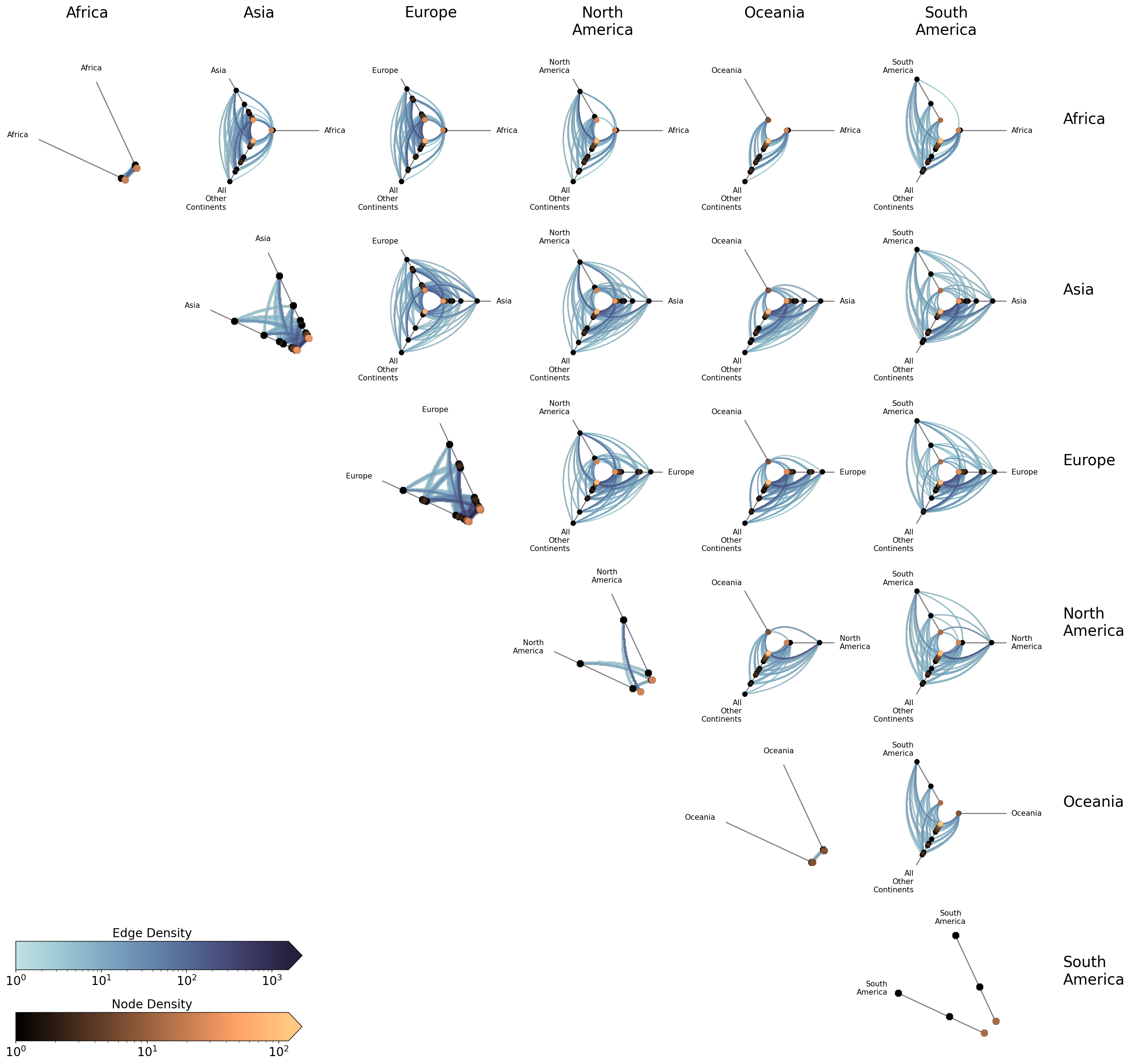
At a glance, we can already see structure in this trade network. Asia, Europe, and North America trade extensively with everyone within this trade group. Africa and Oceania, by contrast, trade minimally within this trade group. The diagonal cells reveal intracontinental trade patterns. Europe’s intragroup trade, for example, is dense while South America’s is nonexistent.

Specifying Partition Values

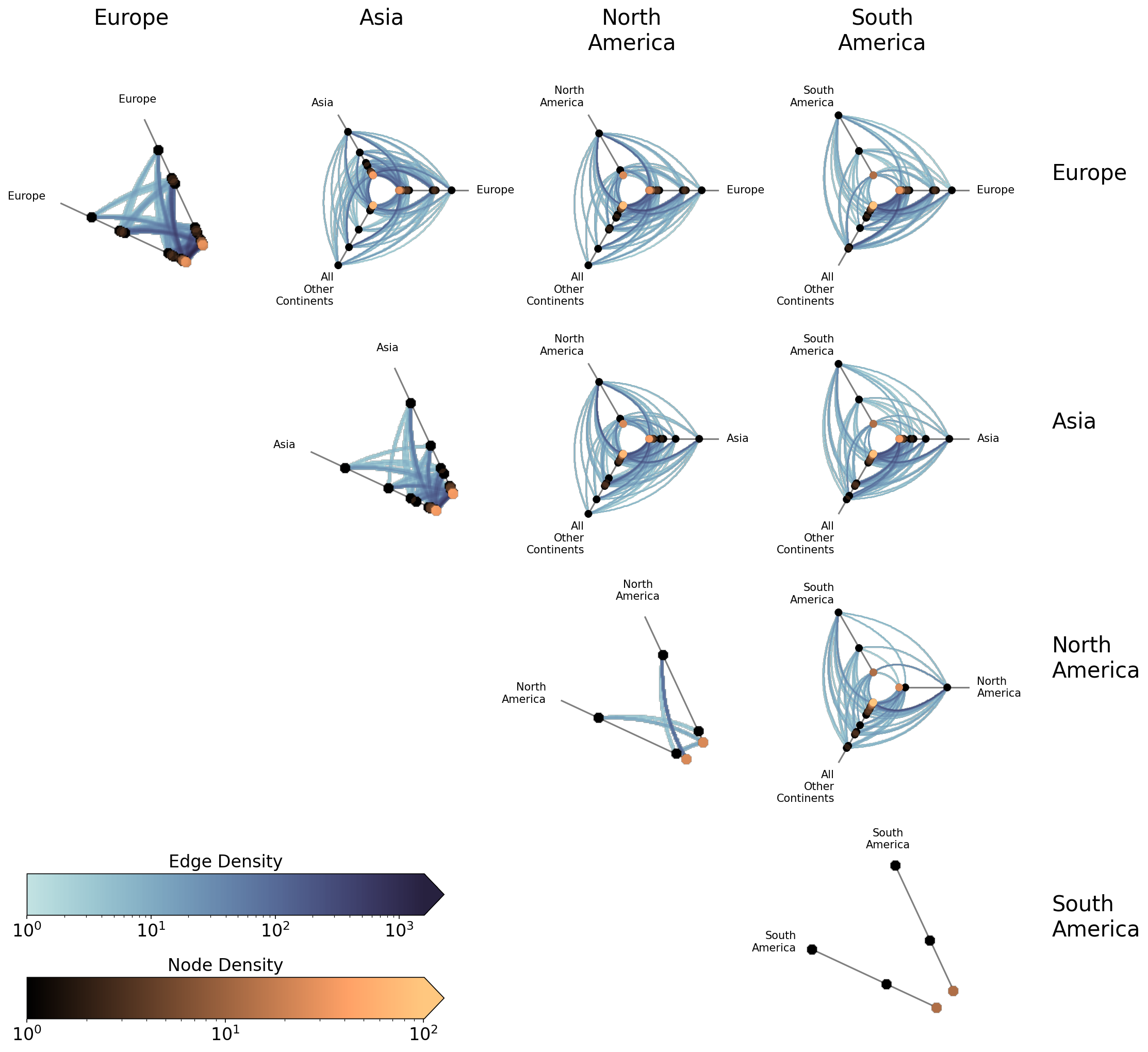
The partition_values parameter gives explicit control over which groups to include and in what order. This is useful for focusing on a subset of groups or for reordering the matrix layout:

hpm_subset = HivePlotMatrix.from_partition(
    nodes=nodes,
    edges=edges,
    partition_variable="continent",
    sorting_variables="export_value",
    partition_values=["Europe", "Asia", "North America", "South America"],
    collapsed_group_axis_name="All Other\nContinents",
    unify_axes=True,
    backend="datashader",
)

hpm_subset.plot()
plt.show()

Excluding Diagonal Cells

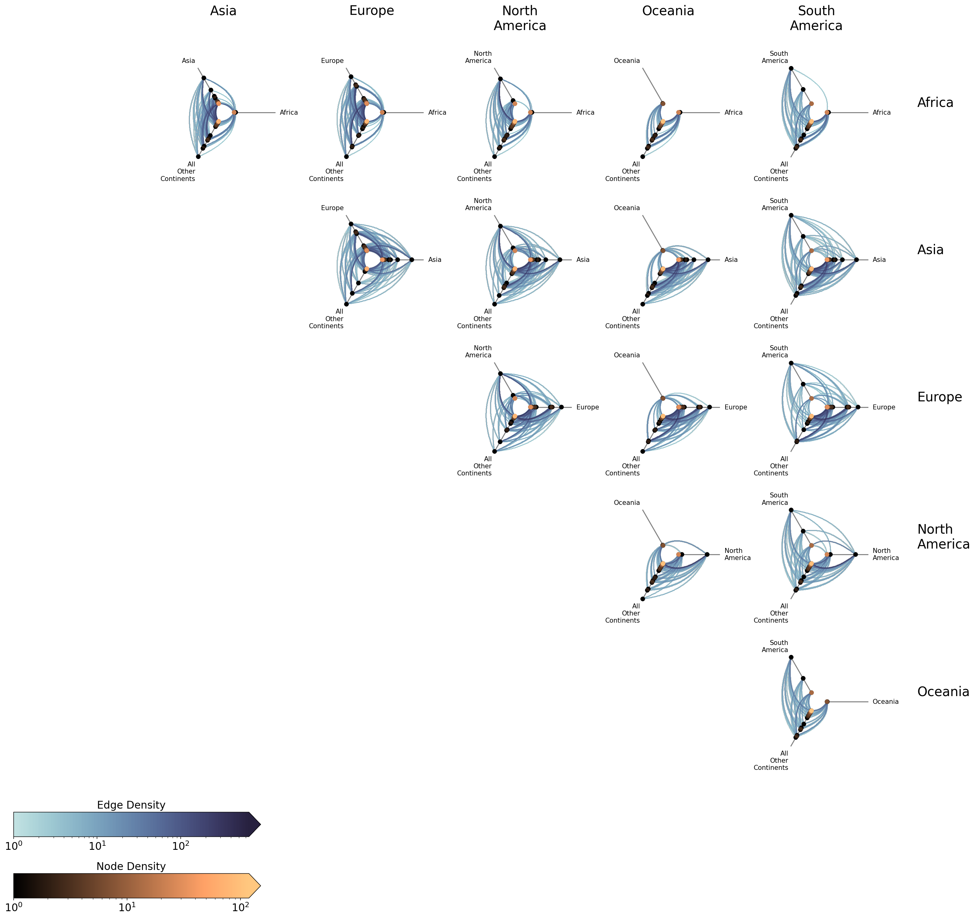
In some cases, we may only care about intergroup relationships and want to exclude the intragroup diagonal cells. This can be done with include_diagonal=False:

hpm_no_diag = HivePlotMatrix.from_partition(
    nodes=nodes,
    edges=edges,
    partition_variable="continent",
    sorting_variables="export_value",
    collapsed_group_axis_name="All Other\nContinents",
    include_diagonal=False,  # skip intragroup diagonal hive plots
    unify_axes=True,
    backend="datashader",
)

hpm_no_diag.plot()
plt.show()

For detailed documentation on using HivePlotMatrix.from_partition(), including visualization back ends, plot options, and styling, see the Hive Plot Matrix From Partition page.

Comparing Sorting and Partition Variables

We now know how to handle networks with many groups, but what if we instead have multiple partition and / or sorting variables to choose from? What if the “right” partition / sorting variable isn’t obvious, and we want to compare several candidates side by side?

The HivePlotMatrix.from_variable_sweep() method makes this easy: it constructs a matrix of hive plots, each using a different sorting variable, partition variable, or both. This allows us to rapidly find network anomalies or structural patterns that only emerge under certain variable choices.

For this section, we will use example_hpm_nodes_and_edges(), generating a toy dataset of 30 nodes in 3 groups with three numeric columns (more on these below).

nodes, edges = example_hpm_nodes_and_edges(edge_tag_counts={"edges": 90})
nodes.data.head()

	unique_id	group	value1	value2	value3
0	0	A	2.579853	7.447622	8.894677
1	1	A	1.462928	9.675097	8.236987
2	2	A	2.861993	3.258254	8.550787
3	3	A	2.324560	3.704597	9.216663
4	4	A	0.313924	4.695558	8.782394

Comparing Sorting Variables

Below, we fix the partition variable and compare three different hive plots side-by-side using three different sorting variables. The three value columns have different relationships for each group:

• value1: correlated with group, so groups will cluster at distinct axis positions.

• value2: uncorrelated noise, so no visible group separation.

• value3: inversely correlated with group (the mirror image of value1).

We also set unify_axes=True so that all cells share the same axis range:

hpm_sorting = HivePlotMatrix.from_variable_sweep(
    nodes=nodes,
    edges=edges,
    partition_variable="group",
    sorting_variables_list=["value1", "value2", "value3"],
    unify_axes=True,
)
hpm_sorting

hiveplotlib.HivePlotMatrix (1 x 3), 3 populated cells, type='from_variable_sweep', backend='matplotlib'

fig, axes = hpm_sorting.plot()
fig.suptitle(
    "Comparing Sorting Variables",
    y=1.1,
)
plt.show()

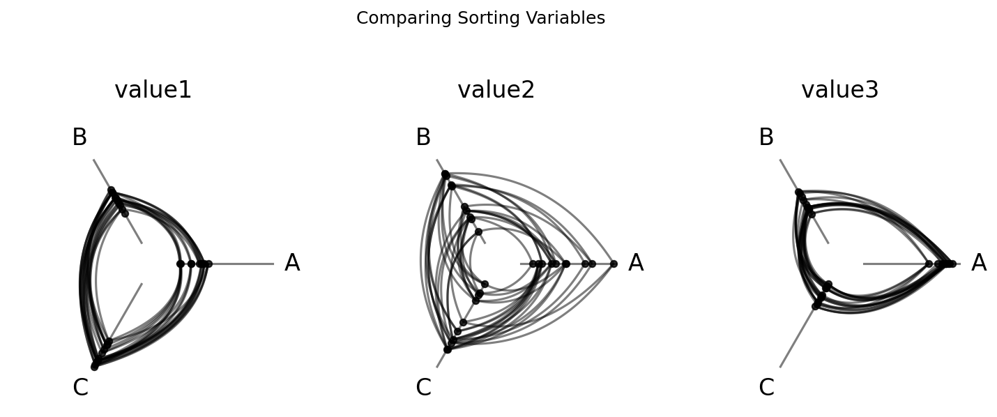
The three panels are visually distinct:

• Sorting by value1 (left) produces clear group clustering: nodes from the same group land at similar axis positions, creating tight, structured edge bundles.

• Sorting by value2 (center) looks noisy and uniform: no group signal in the sort order, so edge bundles spread evenly.

• Sorting by value3 (right) mirrors value1 but inverted: the same clustering structure appears, but groups swap ends on each axis.

This matches what we would expect given the data construction.

Comparing Partition Variables

We can also sweep over different partition variables while keeping the sorting variable fixed. To do this, we need a second partition to compare against the original group labels. The NodeCollection.create_partition_variable() method takes a continuous column and splits it into labeled bins. Here, we divide nodes into Low, Medium, and High cutoffs of value1. (For more on this method, see the Create a Partition Variable page.)

# create a second partition variable: 3-group split based on value1
value1_partition = nodes.create_partition_variable(
    data_column="value1",
    cutoffs=3,
    labels=["Low", "Medium", "High"],
    partition_variable_name="Value1 Partition",
)

hpm_partition = HivePlotMatrix.from_variable_sweep(
    nodes=nodes,
    edges=edges,
    sorting_variables="value1",
    partition_variables_list=[
        "group",
        value1_partition,
    ],  # use new partition variable created above
    unify_axes=True,
)

fig, axes = hpm_partition.plot()
fig.suptitle(
    "Comparing Partition Variables",
    y=1.1,
)
plt.show()

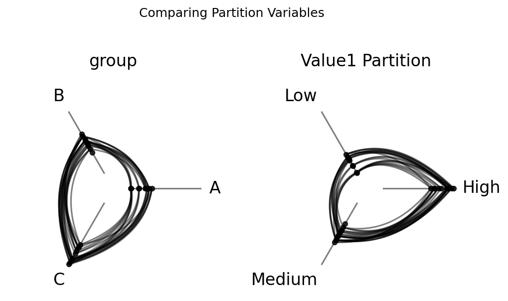
For our right hive plot, we see that the axis labels (Low, Medium, High) directly correspond to where nodes land on each axis, since the partition and sorting variable encode the same information.

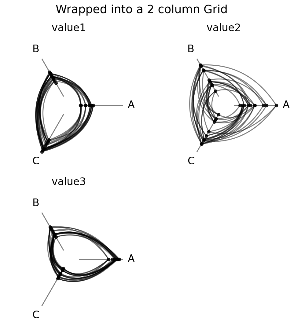
Wrapping with ncols

By default, a single sorting or partition variable sweep will plot as a single-row HPM, but when comparing many variables, a single row can become unwieldy. The ncols parameter wraps the results into multiple rows with ncols columns:

hpm_wrapped = HivePlotMatrix.from_variable_sweep(
    nodes=nodes,
    edges=edges,
    partition_variable="group",
    sorting_variables_list=["value1", "value2", "value3"],
    ncols=2,
    unify_axes=True,
)

fig, axes = hpm_wrapped.plot()
fig.suptitle(
    "Wrapped into a 2 column Grid",
    size=18,
)
plt.show()

2D Grid: Sorting Variables x Partition Variables

What if we want to vary both dimensions at once — sweeping over sorting variables in one direction and partition variables in the other?

When both sorting_variables_list and partition_variables_list are provided, from_variable_sweep() produces a 2D grid where each row corresponds to a different partition variable and each column corresponds to a different sorting variable.

Since we already created the value1 partition above, we can directly build the 2D grid:

hpm_2d = HivePlotMatrix.from_variable_sweep(
    nodes=nodes,
    edges=edges,
    sorting_variables_list=["value1", "value2", "value3"],
    partition_variables_list=["group", value1_partition],
    unify_axes=True,
)

fig, axes = hpm_2d.plot()
fig.suptitle(
    "2D Grid: Partition Variables (rows) x Sorting Variables (columns)",
    size=16,
)
plt.show()

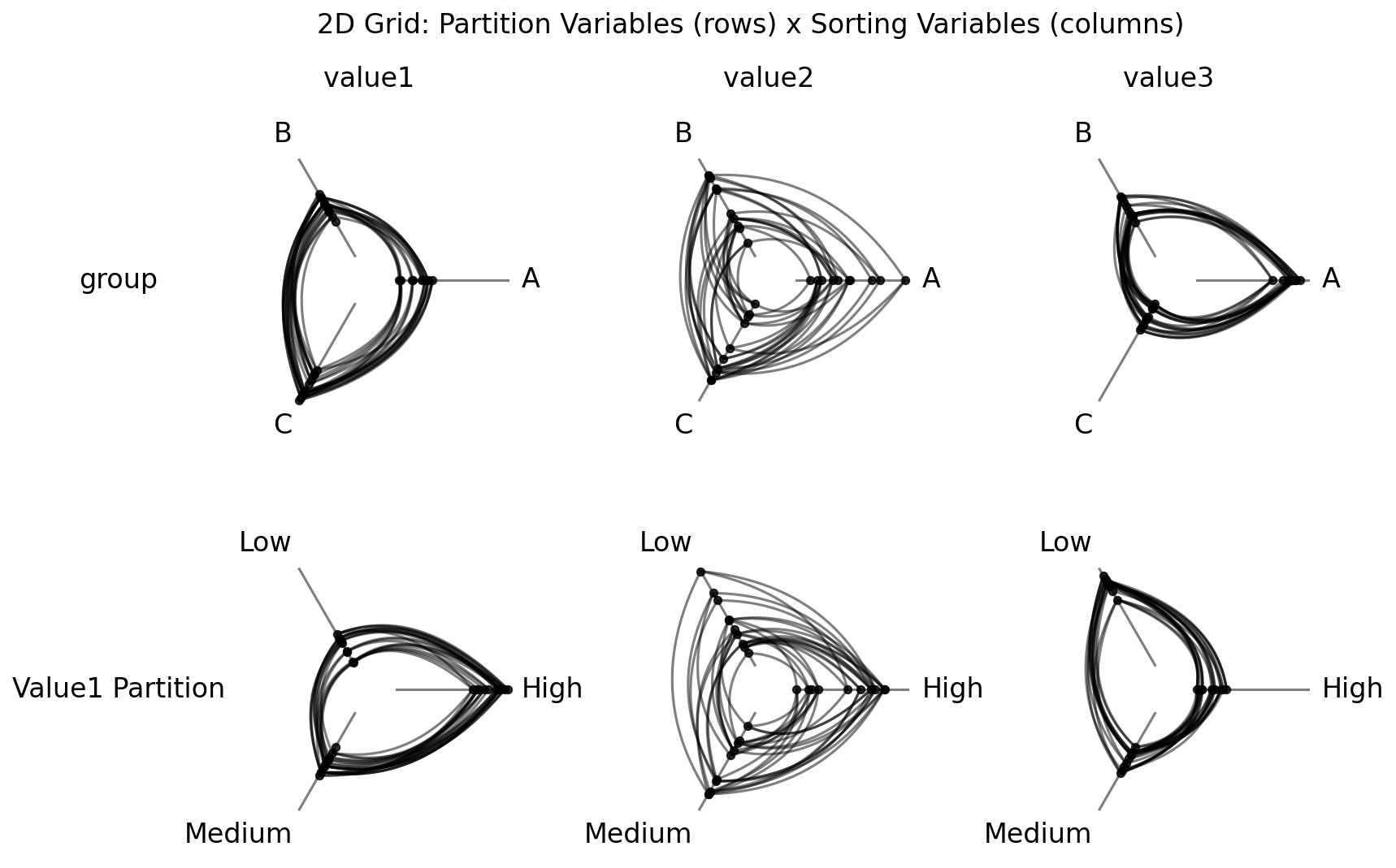
The top row partitions nodes by group label (the ground truth grouping), while the bottom row partitions by the value1 partition. By comparing rows, we can see how different partitioning strategies interact with different sorting variables.

For detailed documentation on using HivePlotMatrix.from_variable_sweep(), including visualization back ends, plot options, and styling, see the Hive Plot Matrix From Variable Sweep page.

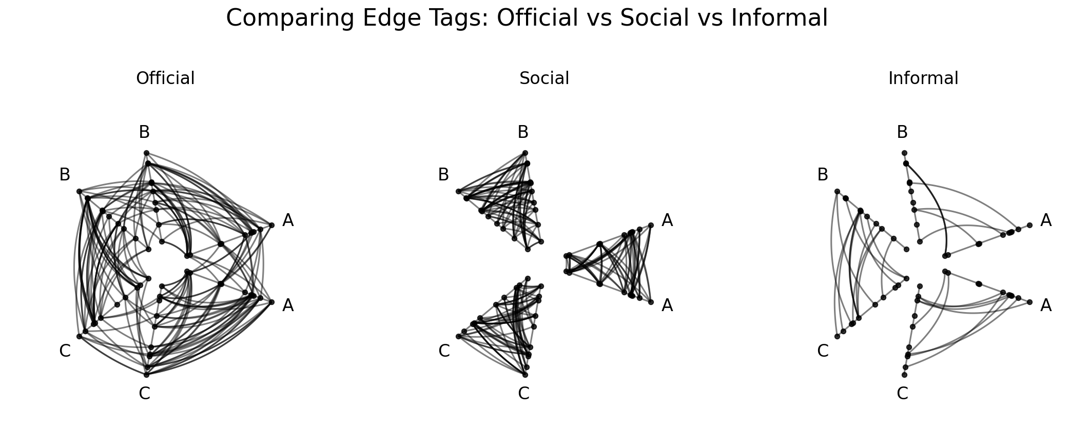
Comparing Edge Tags

Suppose our single network has three distinct types of edge relationships (official, social, and informal), and we suspect that they have different structural properties. If we overlay all three on a single hive plot, they compete for visual attention and confound each other. Instead, we could plot each set of edges in its own hive plot.

That is precisely what HivePlotMatrix.from_tags() is designed for. Given multiple tags of edge data, it constructs one hive plot per tag, letting us compare edge subsets of a single network side by side.

We will generate another toy dataset here, this time with multi-tag edges that have different structural properties: Official edges are random, Social edges are intragroup only, and Informal edges are intergroup only.

nodes_tags, edges_tags = example_hpm_nodes_and_edges(
    edge_tag_counts={"Official": 200, "Social": 200, "Informal": 30},
    edge_structure={"Social": "intragroup", "Informal": "intergroup"},
)
edges_tags

hiveplotlib.Edges of 430 edges across 3 tags.

Below, we first show this network in a single hive plot:

tags_example_single_hp = HivePlot(
    nodes=nodes_tags,
    edges=edges_tags,
    partition_variable="group",
    sorting_variables="value1",
    repeat_axes=True,
)

fig, axes = plt.subplots(1, 2, figsize=(8, 4))

tags_example_single_hp.plot(fig=fig, ax=axes[0])
axes[0].set_title(
    "Single hive plot with all edges\nhides tag-specific differences",
    y=1.1,
)

edges_tags.update_edge_viz_kwargs(tag="Social", color="royalblue")
edges_tags.update_edge_viz_kwargs(tag="Informal", color="darkorange")
tags_example_single_hp = HivePlot(
    nodes=nodes_tags,
    edges=edges_tags,
    partition_variable="group",
    sorting_variables="value1",
    repeat_axes=True,
)

tags_example_single_hp.plot(fig=fig, ax=axes[1])
axes[1].set_title(
    "Tags obscure each other even with color",
    y=1.1,
)
plt.show()

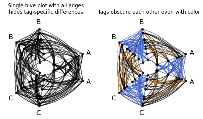
Without color (left), any structural contrast between tags is invisible. Even if we color each tag of edges differently (right), the edge tags still obscure each other, creating misleading patterns at first glance (e.g. no obvious black intragroup edges in the right hive plot above).

By separating them, the HPM immediately reveals a different behavior for each subnetwork:

# we won't need edge tag colors to see things clearly in the HPM
#  so we remove them
edges_tags.update_edge_viz_kwargs(reset_kwargs=True)

hpm_tags = HivePlotMatrix.from_tags(
    nodes=nodes_tags,
    edges=edges_tags,
    partition_variable="group",
    sorting_variables="value1",
    repeat_axes=True,
)

fig, axes = hpm_tags.plot()
fig.suptitle(
    "Comparing Edge Tags: Official vs Social vs Informal",
    size=22,
    y=1.05,
)
plt.show()

With repeat_axes=True, each tag’s hive plot includes repeat axes for all groups, making intragroup edges visible alongside the intergroup edges.

Each plot shows drastically different network activity:

• The Official plot (left) looks random and uniform, with edges spread across all axis pairs with no discernible pattern.

• The Social plot (middle) has exclusively intragroup edges.

• The Informal plot (right), in contrast to Social, has exclusively intergroup edges.

For detailed documentation on using HivePlotMatrix.from_tags(), including visualization back ends, plot options, and styling, see the Hive Plot Matrix From Tags page.

Generic Constructor

The convenience methods cover common use cases, but for other custom arrangements, the generic constructor accepts a list of lists (or dictionary) of HivePlot instances.

Below, we construct a temporal comparison: a network that grows over three years, gaining both new nodes and a wider range of values.

years = [2018, 2019, 2020]
nodes_per_group = [10, 20, 40]
edge_counts = [30, 120, 400]
value_scales = [1, 2, 4]

hive_plots = []

for year, npg, n_edges, scale in zip(
    years, nodes_per_group, edge_counts, value_scales, strict=True
):
    nodes_t, edges_t = example_hpm_nodes_and_edges(
        nodes_per_group=npg,
        edge_tag_counts={"edges": n_edges},
        seed=year,
    )
    # scale the sorting variable so the value range grows over time
    nodes_t.data["value1"] *= scale

    hp = HivePlot(
        nodes=nodes_t,
        edges=edges_t,
        partition_variable="group",
        sorting_variables="value1",
    )
    hive_plots.append(hp)

hpm_custom = HivePlotMatrix(
    hive_plots=[hive_plots],
    col_labels=[str(y) for y in years],
    unify_axes=True,
    backend="datashader",
)
hpm_custom

hiveplotlib.HivePlotMatrix (1 x 3), 3 populated cells, type='generic', backend='datashader'

fig, axes, _, _ = hpm_custom.plot()
fig.suptitle("Network Evolution Over Time", size=18, y=1.05)
plt.show()

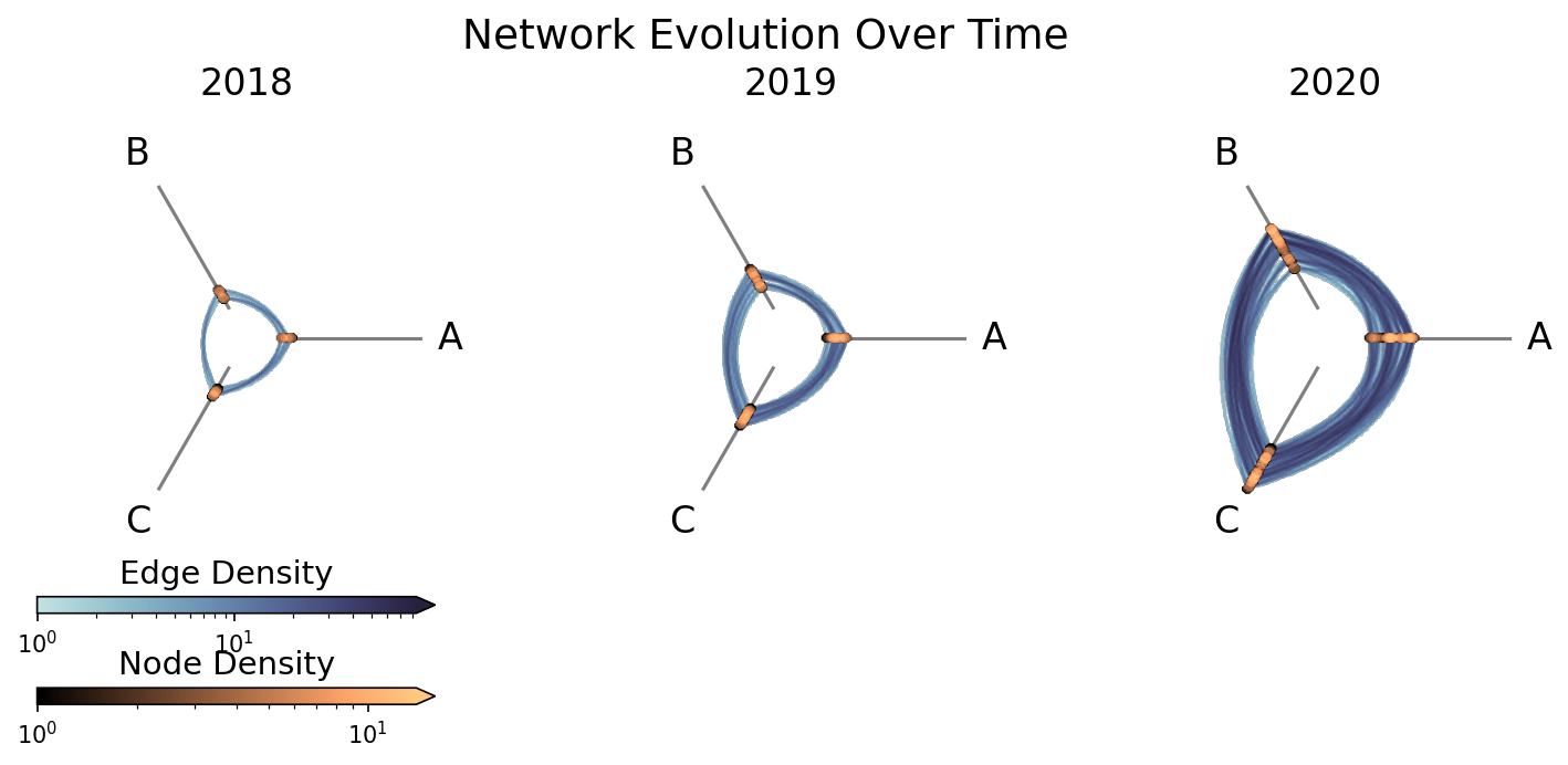
By passing unify_axes=True, all cells share the same axis range, so the growth year-over-year is immediately visible, in particular with nodes moving out on each axis and edge density increasing each year.

For detailed documentation on using HivePlotMatrix generic constructor, including visualization back ends, plot options, and styling, see the Hive Plot Matrix Generic Constructor page.