Hive Plots Using Other Visualization Libraries

This notebook first demonstrates how to visualize hive plots with holoviews, plotly, and bokeh through formal hiveplotlib support.

We then show how to create a baseline JSON output from a toy HivePlot instance.

Next, we use this JSON output to visualize the same toy example in JavaScript using the <hive-plot> Web Component from our sister npm package [@hiveplotlib/d3](https://www.npmjs.com/package/@hiveplotlib/d3).

Finally, we demonstrate how to visualize this toy hive plot in pure matplotlib. Although hiveplotlib of course supports matplotlib visualizations formally, this last example is meant to demonstrate wrangling the JSON data product to help users who need to translate the JSON output to an unsupported Python visualization library.

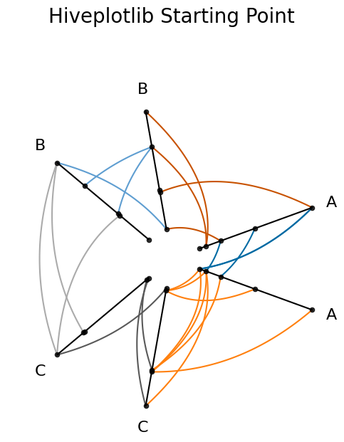
Matplotlib Baseline

We will use the following example throughout this notebook.

import matplotlib.pyplot as plt
from hiveplotlib.datasets import example_hive_plot
from hiveplotlib.utils import cartesian2polar, polar2cartesian

hp = example_hive_plot(
    num_nodes=15,
    num_edges=25,
    repeat_axes=True,
    seed=3,
)

# add some color customization
color_dict = {
    "A": {"A": "#006BA4", "C": "#FF800E"},
    "C": {"B": "#ABABAB", "C": "#595959"},
    "B": {"B": "#5F9ED1", "A": "#C85200"},
}

for p1 in color_dict:
    for p2 in color_dict[p1]:
        hp.update_edges(
            partition_id_1=p1,
            partition_id_2=p2,
            color=color_dict[p1][p2],
        )

fig, ax = hp.plot(
    figsize=(6, 6),
    axes_kwargs={"color": "black", "alpha": 1.0},
    alpha=1,
)
ax.set_title("Hiveplotlib Starting Point", y=1.2, fontsize=20)
plt.show()

For more on the nuances of using the "matplotlib" viz back end, see the Hive Plots in Matplotlib page.

holoviews

hiveplotlib supports visualizations with a holoviews back end. We need only set the viz back end accordingly.

Note: the holoviews-based viz back ends require that hiveplotlib be installed with extra packages, which can be done by running:

pip install hiveplotlib[holoviews]

hiveplotlib supports holoviews plotting using both bokeh ("holoviews-bokeh") and matplotlib ("holoviews-matplotlib").

Holoviews (Bokeh Back End)

hp.set_viz_backend("holoviews-bokeh")

# note the extra plotting kwargs changed to holoviews-bokeh ones, not mpl
fig = hp.plot(
    node_kwargs={"size": 7},
    axes_kwargs={"line_alpha": 1, "line_width": 2},
    line_width=2,
    line_alpha=1,
)
fig = fig.opts(
    title="Hiveplotlib (Holoviews-Bokeh Back End)",
    fontsize={"title": 20},
)
fig

ⓘ

Note that switching to this interactive back end gave us hover information over our nodes, edges, and axes.

For more on the nuances of using the "holoviews-bokeh" viz back end, see the Hive Plots in Holoviews-Bokeh page.

Holoviews (Matplotlib Back End)

hp.set_viz_backend("holoviews-matplotlib")

# note the extra plotting kwargs changed to holoviews-matplotlib ones
fig = hp.plot(
    node_kwargs={"s": 50},
    axes_kwargs={"alpha": 1, "linewidth": 2},
    linewidth=2,
    alpha=1,
)
fig = fig.opts(
    title="Hiveplotlib (Holoviews-Matplotlib Back End)",
    fontsize={"title": 30},
)
fig

ⓘ

For more on the nuances of using the "holoviews-matplotlib" viz back end, see the Hive Plots in Holoviews-Matplotlib page.

bokeh

hiveplotlib supports visualizations with a bokeh back end. We need only set the viz back end accordingly.

Note: the "bokeh" viz back end requires that hiveplotlib be installed with extra packages, which can be done by running:

pip install hiveplotlib[bokeh]

from bokeh.io import output_notebook
from bokeh.plotting import show

output_notebook()

Loading BokehJS ...

hp.set_viz_backend("bokeh")

# note the extra plotting kwargs changed to bokeh ones
fig = hp.plot(
    node_kwargs={"size": 7},
    axes_kwargs={"line_alpha": 1, "line_width": 2},
    line_width=2,
    line_alpha=1,
)
fig.title = "Hiveplotlib (Bokeh Back End)"
fig.title.text_font_size = "30px"
show(fig)

For more on the nuances of using the "bokeh" viz back end, see the Hive Plots in Bokeh page.

plotly

hiveplotlib supports visualizations with a plotly back end. We need only set the viz back end accordingly.

Note: the "plotly" viz back end requires that hiveplotlib be installed with extra packages, which can be done by running:

pip install hiveplotlib[plotly]

import plotly.io

plotly.io.renderers.default = "plotly_mimetype+notebook"

hp.set_viz_backend("plotly")

fig = hp.plot(opacity=1)
fig.update_layout(title="Hiveplotlib (Plotly Back End)", font={"size": 25})
fig

For more on the nuances of using the "plotly" viz back end, see the Hive Plots in Plotly page.

datashader

hiveplotlib supports visualizations with a datashader back end. We need only set the viz back end accordingly.

Note: the "datashader" viz back end requires that hiveplotlib be installed with extra packages, which can be done by running:

pip install hiveplotlib[datashader]

The "datashader" viz back end is for hive plots with large quantities of overlapping nodes and edges, which we will reserve for discussion on the Hive Plots for Large Networks and the the Hive Plots in Datashader pages.

Changing Keyword Arguments When Switching Viz Back End

Keyword arguments with the various back ends (e.g. matplotlib, bokeh) will differ.

Thus, if you have a particular viz back end in mind:

Set your keyword arguments in the context of your plotting tool.

This will be particularly important for keyword arguments like size of nodes and thickness of edges.

Write Keyword Arguments to Generalize When Possible

If you plan to switch between viz back ends, it’s helpful to choose kwargs that standardize between the different viz back ends when possible.

For colors specifically, you can set your colors in a standardized way. Web colors should be preferred here. Conversion to hex codes and RGBA values are easy with the matplotlib.colors.to_hex() and matplotlib.colors.to_rgba() functions.

Changing Kwargs For Viz Back End Compatibility

When changing the viz back end on an existing hive plot, some incompatibilities are unavoidable, notably:

• When the kwarg naming conventions of two viz back ends diverge, then kwarg names must be changed. These kwargs could simply be renamed.

• Some kwargs that exist for one viz back end don’t map onto any kwargs in a different back end. These kwargs must be removed .

Both of these tasks can be easily done with the HivePlot.rename_edge_kwargs() method.

For more on the nuances of switching between viz back ends, see the Changing Visualization Back Ends page.

Exporting Hive Plots as JSON

To accommodate any library / language one might choose for the final visualization of their hive plot, we support exporting the relevant data as JSON via the hiveplotlib.HivePlot.to_json() method.

To pull out the information of this HivePlot instance, we simply need to call the HivePlot.to_json() method.

hp_json = hp.to_json()

What’s in the Output JSON

HivePlot.to_json() creates the following JSON structure:

{
  "axes": {
    "<axis_id_0>": {
      "start": [axis_id_0_start_x (float), axis_id_0_start_y (float)],
      "end": [axis_id_0_end_x (float), axis_id_0_end_y (float)],
      "angle": axis_id_0_angle_degrees (float),
      "long_name": "axis_id_0_long_name (string)",
      "nodes": {
        "unique_id": [list, of, unique, node, ids],
        "x": [list, of, corresponding, node, x, values],
        "y": [list, of, corresponding, node, y, values]
      }
    },
       .
       .
       .
    "<axis_id_n>": {
      ...
    }
  },
  "edges": {
    "from_axis_id": {
      "to_axis_id": {
        "tag": {
          "ids": [
            [from_edge_0, to_edge_0], ... , [from_edge_k, to_edge_k]
          ],
          "curves": [
            [
              [edge_0_x_0, edge_0_y_0], ... , [edge_0_x_j, edge_0_y_j]
            ],
            [
              [edge_1_x_0, edge_1_y_0], ... , [edge_1_x_j, edge_1_y_j]
            ],
            .
            .
            .
            [
              [edge_k_x_0, edge_k_y_0], ... , [edge_k_x_j, edge_k_y_j]
            ]
          ],
          "edge_kwargs": {<edge kwargs>}
        }
      }
    }
  },
  "node_viz_kwargs": {
    "<axis_id_0>": {
      "<kwarg_name>": <scalar value or [per-node list]>,
      ...
    },
    ...
  }
}

The highest-level separation is the top-level keys "axes", "edges", and "node_viz_kwargs".

Axis and Node Information

"axes" contains the start and end points of each axis in Cartesian space, as well as the IDs and corresponding Cartesian coordinates of each node on a given axis.

Each axis entry also includes:

• "angle": the angle of the axis in degrees, which can be used for positioning axis labels.

• "long_name": the human-readable name of the axis, which can be used as a label.

For example, the information about axis "A" is under ["axes"]["A"], and the information for nodes on axis "A" is under:

["axes"]["A"]["nodes"].

Edge Information

"edges" contains the discretized curve information for plotting edges. Organized by nested dictionaries, the edges that go from axis "A" to axis "B" are stored under:

["edges"]["A"]["B"].

The underlying curve information will be nested one layer deeper under the “tag” of data being referenced. For more on tags, see the discussion on comparing subgroups in a single hive plot. Note, if you have not concerned yourself with tags up to this point, your tag will likely be "0".

All discretized curves that go from axis "A" to axis "B" are stored under:

["edges"]["A"]["B"][<tag>]["curves"]

where the \(n^{th}\) curve’s data is contained under:

["edges"]["A"]["B"][<tag>]["curves"][n].

One can also pull the corresponding node IDs from and to which each edge is being drawn under:

["edges"]["A"]["B"][<tag>]["ids"]

where, similarly, the the \(n^{th}\) pair of node IDs corresponding to the \(n^{th}\) curve is contained under:

["edges"]["A"]["B"][<tag>]["ids"][n].

Any corresponding edge kwargs generated along the way are preserved under:

["edges"]["A"]["B"][<tag>]["edge_kwargs"].

Node Visualization Kwargs

"node_viz_kwargs" contains per-axis node styling information. If node visualization kwargs were set on the HivePlot instance (e.g. via HivePlot.update_node_viz_kwargs()), they will appear here keyed by axis name.

For kwargs whose values reference a column in the node data (e.g. c="my_column"), the values are resolved to per-node lists matching the ordering of nodes in the corresponding axis entry. Scalar kwargs (e.g. s=20) are preserved as-is.

JavaScript Viz from JSON

Once we have a standardized format like JSON, we need not even restrict ourselves to Python.

We need only save the JSON string output to disk, then we can load the resulting .json file in any programming language.

The JSON output can be saved by running:

with open('my_hive_plot.json', 'w') as f:
    f.write(hp_json)

Below, we use the [@hiveplotlib/d3](https://www.npmjs.com/package/@hiveplotlib/d3) npm package to visualize the JSON output in JavaScript via its <hive-plot> Web Component.

The <hive-plot> Web Component renders SVG elements with semantic CSS classes (.node, .edge, .axis, .axis-label) and data-* attributes (e.g. data-axis, data-node-id, data-source-axis, data-target-axis, data-tag), making it easy to customize the visualization with plain CSS. Below, we demonstrate thickening nodes and edges on hover.

Note, below we plot the saved JSON file from the hiveplotlib-javascript repository, which is equivalent to our above example, but one could also pass the local file path (e.g. src="my_hive_plot.json") if working locally.

import IPython.display

js_url = (
    "https://cdn.jsdelivr.net/npm/@hiveplotlib/d3/hive_plot_element.min.js"
)

hp_json_file_url = (
    "https://raw.githubusercontent.com/gjkoplik/"
    "hiveplotlib-javascript/main/example_hive_plot.json"
)

script = f"""
<div> <h1> Hive Plots in JavaScript </h1> </div>

<script type="module" src="{js_url}"></script>

<style>
    .edge:hover {{
        stroke-width: 5;
    }}
    .node:hover {{
        r: 5;
    }}
</style>

<hive-plot src="{hp_json_file_url}"></hive-plot>
"""

IPython.display.display(IPython.display.HTML(script))

Hive Plots in JavaScript

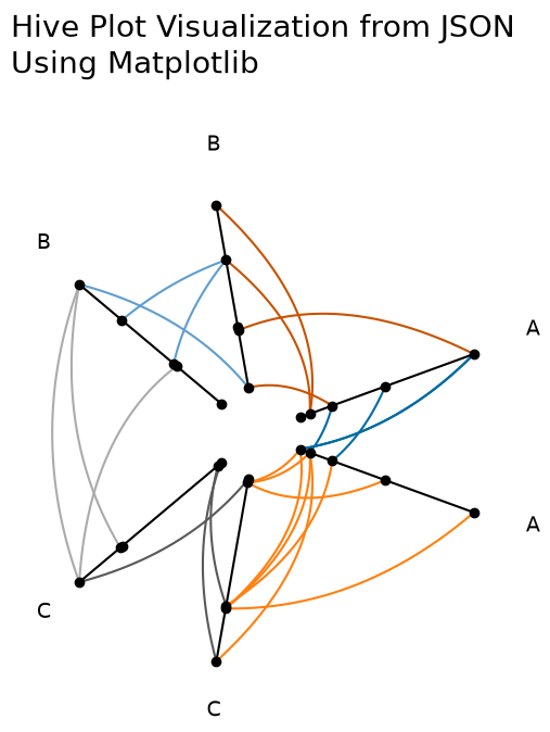
Replicating our Matplotlib Viz from JSON

Once we read the JSON back into Python as a dict, we can manually plot in matplotlib without touching any hiveplotlib-specific visualization functions.

Although hiveplotlib of course supports matplotlib visualizations formally, this last example is meant to demonstrate wrangling the JSON data product to help users who need to translate the JSON output to a different Python visualization library.

import json

import matplotlib.pyplot as plt
import numpy as np
from matplotlib.collections import LineCollection

%matplotlib inline

# read in JSON output that we exported from `HivePlot` instance above
hp_dict = json.loads(hp_json)

fig, ax = plt.subplots(figsize=(6, 6))

for axis in hp_dict["axes"]:
    # plot axis
    axis_start = hp_dict["axes"][axis]["start"]
    axis_end = hp_dict["axes"][axis]["end"]
    axis_range = np.vstack([axis_start, axis_end])
    ax.plot(axis_range[:, 0], axis_range[:, 1], color="black")

    # plot nodes
    nodes = hp_dict["axes"][axis]["nodes"]
    ax.scatter(nodes["x"], nodes["y"], color="black", zorder=2)

    # add axis labels using long_name and angle from JSON
    label = hp_dict["axes"][axis].get("long_name", axis)
    rho, phi = cartesian2polar(x=axis_end[0], y=axis_end[1])
    new_x, new_y = polar2cartesian(rho=rho + 1.2, phi=phi)
    ax.text(s=label, x=new_x, y=new_y, size=14)

# plot edges
for edge_from in hp_dict["edges"]:
    for edge_to in hp_dict["edges"][edge_from]:
        for tag in hp_dict["edges"][edge_from][edge_to]:
            # only plot if there are curves generated
            if "curves" in hp_dict["edges"][edge_from][edge_to][tag]:
                curves_to_plot = [
                    np.array(i).astype(float)
                    for i in hp_dict["edges"][edge_from][edge_to][tag][
                        "curves"
                    ]
                ]
                color = hp_dict["edges"][edge_from][edge_to][tag][
                    "edge_kwargs"
                ]["color"]
                # if there's no actual edges there, don't plot
                if len(curves_to_plot) > 0:
                    collection = LineCollection(
                        curves_to_plot, zorder=1, color=color
                    )
                    ax.add_collection(collection)


ax.set_title(
    "Hive Plot Visualization from JSON\nUsing Matplotlib",
    x=0,
    y=1.2,
    size=20,
    ha="left",
)
ax.axis("off")
ax.axis("equal")
plt.show()