Create a Partition Variable

Hive plots require a partition of nodes onto a set of axes.

This page discusses how Hiveplotlib supports rapidly and flexibly creating partition variables in a hiveplotlib.NodeCollection instance via the NodeCollection.create_partition_variable() method. The resulting partition can be used to assign nodes to axes in a hive plot.

import matplotlib.pyplot as plt
import seaborn as sns
from hiveplotlib import HivePlot
from hiveplotlib.datasets import example_edges, example_node_collection

We will base this discussion on the following example NodeCollection:

base_nodes = example_node_collection()
base_nodes.data

	unique_id	low	med	high
0	0	6.363247	14.795079	23.193620
1	1	2.695169	12.321405	21.873202
2	2	0.409326	18.010787	26.718541
3	3	0.165111	19.226066	21.949123
4	4	8.124570	12.658641	25.771102
...	...	...	...	...
95	95	9.562530	15.708242	25.857141
96	96	1.486152	10.064025	21.225680
97	97	9.716562	17.718766	29.328351
98	98	8.890456	19.772874	26.833664
99	99	8.215515	15.892802	28.229576

100 rows × 4 columns

Basic Functionality

We create a node partition via the NodeCollection.create_partition_variable() method.

This method builds a partition based on a column of data in the NodeCollection.data dataframe attribute.

We can also modify how we split the partition groups as well as how we label the partition.

Each generated partition variable will be stored in the NodeCollection.data attribute as another dataframe column.

# keep our examples distinct from each other
nodes = base_nodes.copy()

# default partitions into 3 bins
partition_column_name = nodes.create_partition_variable(
    data_column="low",
    labels=["A", "B", "C"],  # results in cleaner hive plot axes labels
)

nodes.data.head()

	unique_id	low	med	high	partition_0
0	0	6.363247	14.795079	23.193620	B
1	1	2.695169	12.321405	21.873202	A
2	2	0.409326	18.010787	26.718541	A
3	3	0.165111	19.226066	21.949123	A
4	4	8.124570	12.658641	25.771102	C

We can then use this new partition column as the partition_variable in a HivePlot instance:

edges = example_edges(nodes=nodes)

hp = HivePlot(
    nodes=nodes,
    edges=edges,
    partition_variable=partition_column_name,  # created above
    sorting_variables="low",
)

hp.plot();

Below, we go into greater detail about the options for the NodeCollection.create_partition_variable() method.

Data Column

The one required parameter for the NodeCollection.create_partition_variable() method is data_column. This dictates which column to use from the NodeCollection.data dataframe to generate the partition. More on this in the “Cutoffs” section below.

Cutoffs

Once we choose which data_column to use for our partition, we must choose our partition cutoffs. This will dictate how we bin node values from the data_column.

Integer Cutoffs

By choosing an integer for the cutoffs parameter, we will partition the chosen data_column into that many equally sized bins.

Below, we partition the low column into 3 bins.

# keep our examples distinct from each other
nodes = base_nodes.copy()


# this is also the default value for `cutoffs`
cutoffs = 3

partition_column_name = nodes.create_partition_variable(
    data_column="low",
    cutoffs=cutoffs,
)

nodes.data.head()

	unique_id	low	med	high	partition_0
0	0	6.363247	14.795079	23.193620	(3.912, 7.288]
1	1	2.695169	12.321405	21.873202	(0.0264, 3.912]
2	2	0.409326	18.010787	26.718541	(0.0264, 3.912]
3	3	0.165111	19.226066	21.949123	(0.0264, 3.912]
4	4	8.124570	12.658641	25.771102	(7.288, 9.962]

fig, axes = plt.subplots(1, 2, figsize=(9, 3))

# set hue order to match colors between 2 plots
hue_order = sorted(nodes.data[partition_column_name].unique())

sns.stripplot(
    data=nodes.data,
    x="low",
    hue=partition_column_name,
    ax=axes[0],
    hue_order=hue_order,
    legend=False,
)

sns.countplot(
    data=nodes.data,
    x=partition_column_name,
    hue=partition_column_name,
    ax=axes[1],
    hue_order=hue_order,
)

sns.move_legend(
    axes[1],
    "lower center",
    bbox_to_anchor=(-0.1, -0.5),
    ncol=3,
    title="Partition",
    frameon=False,
)

fig.suptitle(
    "Partition on Node Variable 'low'"
    f"\nDefault cutoffs={cutoffs} Results in Equal-Sized Bins",
    y=1.1,
)
plt.show()

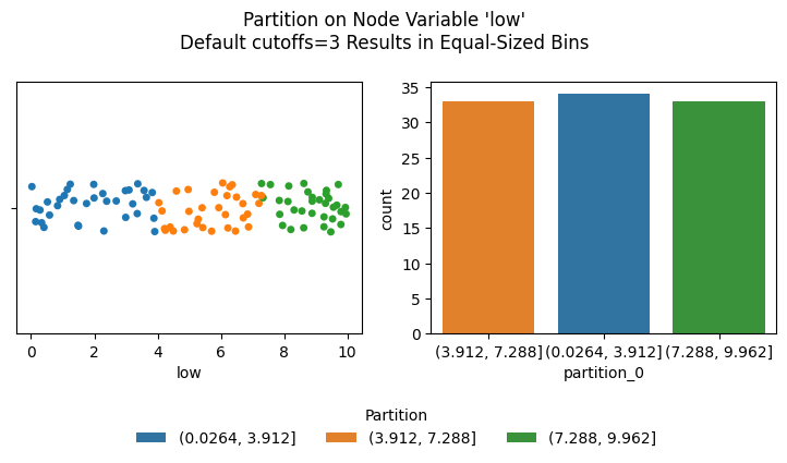
Note, by default the partition names here are the numerical ranges of each partition. These can be renamed via the labels parameter, discussed further below.

List Cutoffs

We can also create explicit cutoffs by providing a list input when partitioning numerical data. This can be useful when specific cutoffs create a more meaningful partition of groups in the downstream hive plot.

Below, we partition the low column into 3 bins, but this time by specifying 2 specific cutoff points.

# keep our examples distinct from each other
nodes = base_nodes.copy()

# 2 cutoffs => 3 bins
cutoffs = [2, 5]

partition_column_name = nodes.create_partition_variable(
    data_column="low",
    cutoffs=cutoffs,
)

nodes.data.head()

	unique_id	low	med	high	partition_0
0	0	6.363247	14.795079	23.193620	(5.0, inf]
1	1	2.695169	12.321405	21.873202	(2.0, 5.0]
2	2	0.409326	18.010787	26.718541	(-inf, 2.0]
3	3	0.165111	19.226066	21.949123	(-inf, 2.0]
4	4	8.124570	12.658641	25.771102	(5.0, inf]

fig, ax = plt.subplots()

sns.stripplot(
    data=nodes.data,
    x="low",
    hue=partition_column_name,
    ax=ax,
)

for cutoff in cutoffs:
    ax.axvline(x=cutoff, color="black", ls="--")

ax.set_title(f"Partition on Node Variable 'low'\ncutoffs={cutoffs}")
plt.show()

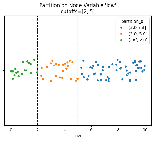
Note, by default the partition names here are the numerical ranges of each partition. These can be renamed via the labels parameter, discussed further below.

Labels

The labels used for the partition will eventually become our default hive plot axis names. Although these can be changed later (via the HivePlot.update_axis() call, see the Modifying Axes page for more), we can easily name them as desired here with the labels parameter.

Default Labels

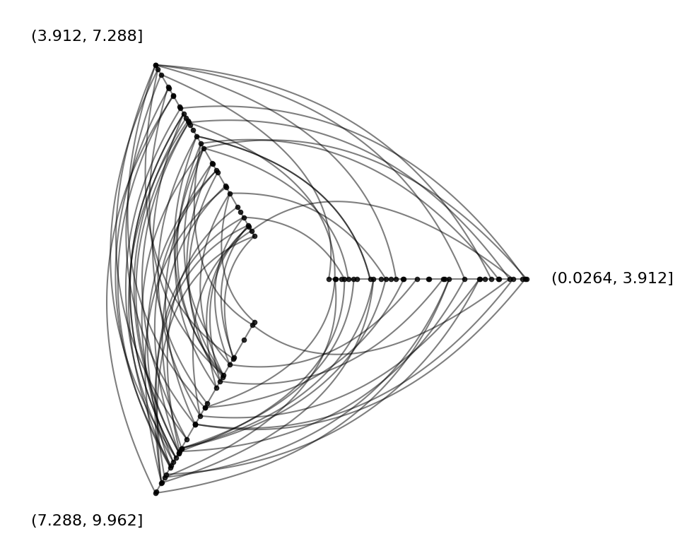
By default, the partition names are the numerical ranges of each partition:

# keep our examples distinct from each other
nodes = base_nodes.copy()

# default partitions into 3 bins
partition_column_name = nodes.create_partition_variable(
    data_column="low",
)

nodes.data.head()

	unique_id	low	med	high	partition_0
0	0	6.363247	14.795079	23.193620	(3.912, 7.288]
1	1	2.695169	12.321405	21.873202	(0.0264, 3.912]
2	2	0.409326	18.010787	26.718541	(0.0264, 3.912]
3	3	0.165111	19.226066	21.949123	(0.0264, 3.912]
4	4	8.124570	12.658641	25.771102	(7.288, 9.962]

edges = example_edges(nodes=nodes)

hp = HivePlot(
    nodes=nodes,
    edges=edges,
    partition_variable=partition_column_name,  # created above
    sorting_variables="low",
)

hp.plot();

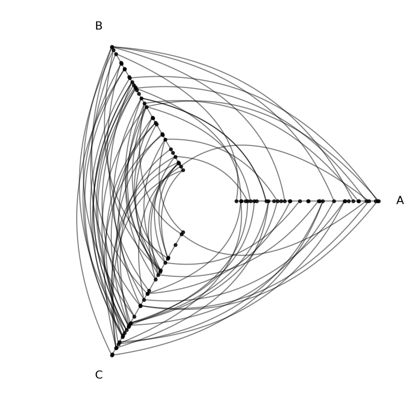
Custom Labels

By providing custom labels values (one label per unique value in the partition column), we can create more readable hive plot axes in the downstream hive plot visualization.

# keep our examples distinct from each other
nodes = base_nodes.copy()

# default partitions into 3 bins
partition_column_name = nodes.create_partition_variable(
    data_column="low",
    labels=["A", "B", "C"],  # becomes more readable hive plot axes labels
)

nodes.data.head()

	unique_id	low	med	high	partition_0
0	0	6.363247	14.795079	23.193620	B
1	1	2.695169	12.321405	21.873202	A
2	2	0.409326	18.010787	26.718541	A
3	3	0.165111	19.226066	21.949123	A
4	4	8.124570	12.658641	25.771102	C

edges = example_edges(nodes=nodes)

hp = HivePlot(
    nodes=nodes,
    edges=edges,
    partition_variable=partition_column_name,  # created above
    sorting_variables="low",
)

hp.plot();

Partition Variable Name

The resulting partition variable column will be named by default in the NodeCollection.data dataframe, but if we choose, we can set it to a custom name. We consider both cases below.

Default Partition Variable Name

By default, these names will increment partition_0, partition_1, etc. as we generate more partitions, ensuring that the column name is different from all exisiting columns in NodeCollection.data:

# keep our examples distinct from each other
nodes = base_nodes.copy()

# make multiple partitions
low_partition_column_name = nodes.create_partition_variable(
    data_column="low",
)

med_partition_column_name = nodes.create_partition_variable(
    data_column="med",
)

nodes.data.head()

	unique_id	low	med	high	partition_0	partition_1
0	0	6.363247	14.795079	23.193620	(3.912, 7.288]	(13.69, 17.185]
1	1	2.695169	12.321405	21.873202	(0.0264, 3.912]	(10.063, 13.69]
2	2	0.409326	18.010787	26.718541	(0.0264, 3.912]	(17.185, 19.939]
3	3	0.165111	19.226066	21.949123	(0.0264, 3.912]	(17.185, 19.939]
4	4	8.124570	12.658641	25.771102	(7.288, 9.962]	(10.063, 13.69]

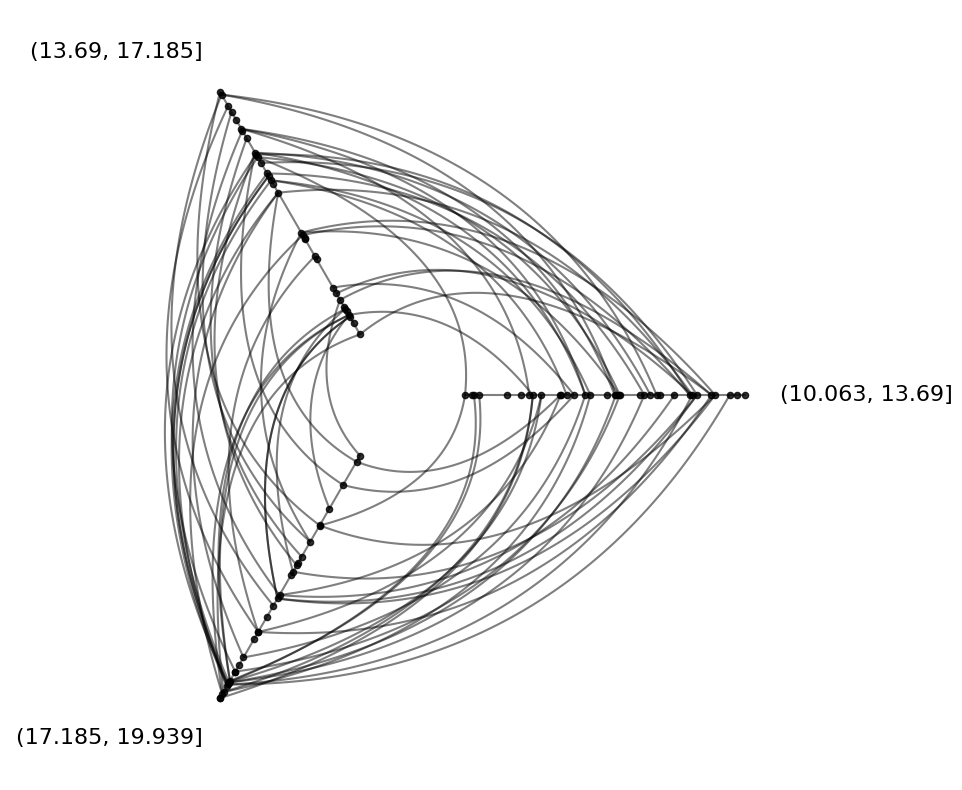
Furthermore, the NodeCollection.create_partition_variable() method returns the resulting partition column name, allowing us to store that name to pass to the downstream HivePlot instance as its partition_variable input:

# name of med partition column was stored above
med_partition_column_name

'partition_1'

edges = example_edges(nodes=nodes)

# use partition on 'med' made above
hp = HivePlot(
    nodes=nodes,
    edges=edges,
    partition_variable=med_partition_column_name,  # created above
    sorting_variables="low",
)

hp.plot();

Custom Partition Variable Name

If we prefer a custom name for our resulting partition variables, we can instead explicitly set the partition_variable_name:

# keep our examples distinct from each other
nodes = base_nodes.copy()

my_custom_partition_name = "Custom Partition Name"

# this call still returns `my_custom_partition_name`
nodes.create_partition_variable(
    data_column="low",
    partition_variable_name=my_custom_partition_name,
)

nodes.data.head()

	unique_id	low	med	high	Custom Partition Name
0	0	6.363247	14.795079	23.193620	(3.912, 7.288]
1	1	2.695169	12.321405	21.873202	(0.0264, 3.912]
2	2	0.409326	18.010787	26.718541	(0.0264, 3.912]
3	3	0.165111	19.226066	21.949123	(0.0264, 3.912]
4	4	8.124570	12.658641	25.771102	(7.288, 9.962]

Using a Subset of Partition Values

By default, each partition value will become an axis in the downstream hive plot, but maybe you don’t want to include all of these axes in the final hive plot.

This can be resolved in the HivePlot instance by setting its axes_order to a subset of partition values. For more information, see the Changing Axis Order page.

Collapsing Partition Values Onto a Single Axis

If you want to collapse multiple partition values onto a single axis, particularly if you have a partition with more than 4 values, this can be done within a HivePlot instance. For more information, see the Collapsing Axes page.