Exporting Hive Plots to NetworkX

The HivePlot.to_networkx() method converts a hive plot’s underlying nodes and edges into a networkx graph.

This notebook demonstrates the default exporting functionality, supported output graph types, and how multi-tag edges are exported.

Note: this notebook requires that Hiveplotlib be installed with extra packages, which can be done by running:

pip install hiveplotlib[networkx]

import matplotlib.pyplot as plt
import networkx as nx
from hiveplotlib.datasets import (
    example_hive_plot,
    example_multi_tag_hive_plot,
)

We will base our initial export demonstration on the following toy hive plot:

hp = example_hive_plot(
    num_nodes=15,
    num_edges=25,
    repeat_axes=True,
    seed=3,
)
# data-dependent node and edge coloring
hp.update_edge_plotting_keyword_arguments(
    array="low",
    cmap="Blues",
    clim=(0, 10),
)
hp.update_node_viz_kwargs(
    c="low",
    s=30,
    alpha=0.8,
    edgecolor="black",
    vmin=0,
    vmax=10,
    cmap="Reds",
)

fig, ax = hp.plot(
    figsize=(6, 6),
    alpha=1,
)
ax.set_title("Hiveplotlib Starting Point", y=1.2, fontsize=20)
plt.show()

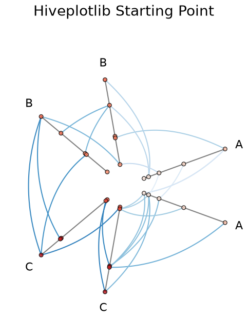
The hive plot’s underlying nodes and edges are the basis for the exported graph:

hp.nodes.data.head()

	unique_id	low	med	high	partition_0
0	0	0.855635	19.553110	23.738696	A
1	1	2.365737	12.839170	20.907619	A
2	2	8.004732	16.478987	26.598396	C
3	3	5.815799	16.955198	29.305324	C
4	4	0.940345	12.924280	22.069840	A

hp.edges.data.head()

	from	to	low	med	high
0	12	1	3.333855	15.282103	23.864390
1	2	3	6.910265	16.717092	27.951860
2	2	12	6.153353	17.102012	26.709778
3	13	8	6.600272	11.719938	27.703492
4	0	1	1.610686	16.196140	22.323157

Default Export

HivePlot.to_networkx() returns a networkx.MultiDiGraph by default. The defaults assume directed edges (matching the (from, to) semantics of the Edges class) and preserve duplicate edges as parallel edges in the resulting graph:

G = hp.to_networkx()
type(G)

networkx.classes.multidigraph.MultiDiGraph

Non-unique_id columns from the NodeCollection shown above and non-from/to columns from each tag’s edge DataFrame are carried over as node and edge attributes on the resulting graph:

# pull a representative node and edge to inspect the carried-over attributes
sample_node = next(iter(G.nodes(data=True)))
sample_edge = next(iter(G.edges(data=True)))
print("node:", sample_node)
print("edge:", sample_edge)

node: (0, {'low': 0.8556351797648074, 'med': 19.553109875812623, 'high': 23.738695896449922, 'partition_0': 'A'})
edge: (0, 1, {'low': 1.6106860703299217, 'med': 16.196139750831524, 'high': 22.32315725217873})

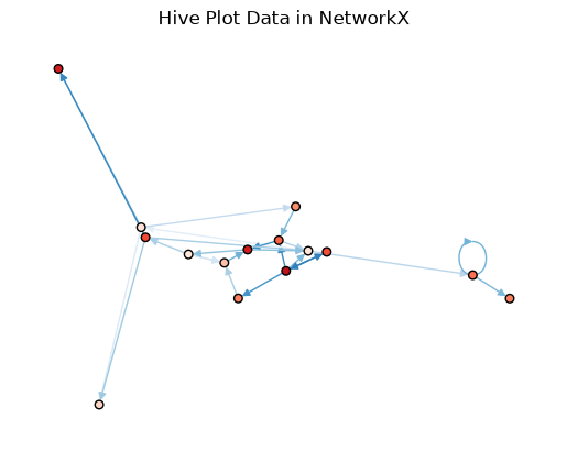
Since the "low" variables in both node and edge data have been carried over to the resulting NetworkX graph, we can still plot with comparable node and edge colors via nx.draw().

Hiveplotlib’s plotting kwargs for nodes and edges are not carried over in the export, so we will set node_color and edge_color manually on the networkx side:

# color nodes by node "low" value
node_values = [data["low"] for node, data in G.nodes(data=True)]

# color edges by edge "low" value
edge_values = [data["low"] for u, v, data in G.edges(data=True)]

# consistent spring layout
pos = nx.spring_layout(G, seed=0)

fig, ax = plt.subplots()
nx.draw(
    G,
    pos=pos,
    edge_color=edge_values,
    edge_cmap=plt.cm.Blues,
    edge_vmin=0,
    edge_vmax=10,
    node_size=30,
    edgecolors="black",  # node edge color
    node_color=node_values,
    vmin=0,
    vmax=10,
    cmap="Reds",
    ax=ax,
)
ax.set_title("Hive Plot Data in NetworkX")
plt.show()

Choosing the Output Graph Type

Two boolean parameters in HivePlot.to_networkx(), directed and multigraph, control the type of the returned NetworkX graph:

directed	multigraph	return type
True (default)	True (default)	networkx.MultiDiGraph
True	False	networkx.DiGraph
False	True	networkx.MultiGraph
False	False	networkx.Graph

Setting directed=False will treat the edges as undirected. Setting multigraph=False will silently merge duplicate (from, to) rows into a single edge (last write wins).

Multi-Tag Edges

If the underlying Edges instance has more than one tag, then the tag information is written into each networkx edge as an attribute named "tag" in the resulting graph.

(Single-tag inputs do not write a "tag" attribute.)

We will construct a small two-tag example to demonstrate:

hp_multi = example_multi_tag_hive_plot()

fig, ax = hp_multi.plot(figsize=(6, 6))
ax.set_title("Hiveplotlib Multi-Tag Starting Point", y=1.2, fontsize=20)
plt.show()

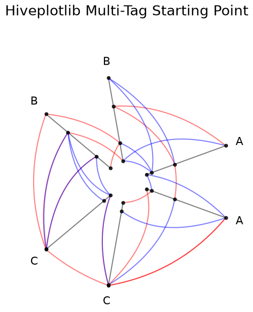
After exporting to networkx, the "tag" attribute is created for each edge:

G_multi = hp_multi.to_networkx()

# every edge in the multigraph carries its source tag
for u, v, data in list(G_multi.edges(data=True))[:5]:
    print(f"({u}, {v}) tag={data['tag']!r}")

(0, 5) tag='tag_red'
(0, 4) tag='tag_red'
(0, 1) tag='tag_blue'
(1, 1) tag='tag_red'
(2, 9) tag='tag_red'

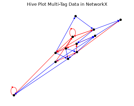
We can use the "tag" edge attribute to set edge_color on the networkx side, just as we did with "low" in the previous example, when calling nx.draw():

tag_colors = {"tag_red": "red", "tag_blue": "blue"}

# color edges by tag value
edge_colors = [
    tag_colors[data["tag"]]
    for u, v, key, data in G_multi.edges(keys=True, data=True)
]

# consistent spring layout
pos = nx.spring_layout(G_multi, seed=0)

fig, ax = plt.subplots()
nx.draw(
    G_multi,
    pos=pos,
    edge_color=edge_colors,
    node_size=30,
    node_color="black",
    ax=ax,
)
ax.set_title("Hive Plot Multi-Tag Data in NetworkX")
plt.show()

For more on exporting to JSON for use in other languages or visualization libraries, see the Exporting Hive Plots to JSON page.

For more on building a HivePlot from a networkx graph, see the Creating Hive Plots from NetworkX page.

For more on computing graph metrics on the underlying nodes and edges, see the Computing Graph Metrics page.